p <- K93_Individual()

# 3 parameters
p$ode_size
[1] 3# size, mortality and fecundity
p$ode_names[1] "height" "mortality" "fecundity"# initialised at 2 cm DBH
p$ode_state[1] 2 0 0# set to fixed state
p$ode_state <- c(50, 0, 0)Kohyama 1993 — the forest architecture hypothesis for the stable coexistence of species
model
This page builds on The big picture. Read it first if the notation here is unfamiliar.
Imagine a forest where every tree of a given size behaves the same way, regardless of species. A tree’s diameter alone tells you roughly how fast it grows, how likely it is to die, and how many offspring it produces, once you also account for how much basal area — a proxy for crowding — sits above it in the canopy. That is the whole idea behind the K93 model: growth, mortality, and fecundity are simple, size-dependent rules shaped by competition from larger neighbours, not by any species-specific strategy.
This is a deliberately different starting point from the trait-based FF16 model described elsewhere in this documentation. FF16 asks what an individual plant should do given its own physiological traits, such as leaf economics or wood density, and derives vital rates from first principles. K93 instead asks what pattern of vital rates, fitted directly to size and competition, allows many species to coexist in a stand over the long run. It is a statistical description of a forest rather than a mechanistic model of a plant. The rest of this page makes this precise.
This document outlines the K93 physiological model used in the plant package. This model was first described, and has primarily been developed, elsewhere, in particular in Kohyama (1993). The model’s equations are presented here not as original findings, but rather so that users can understand the full system of equations being solved within plant.
The purpose of a physiological model in plant is to take a plant’s current size, light environment, and physiological parameters as inputs, and return its growth, mortality, and fecundity rates. In the K93 physiological model, these vital rates are all estimated using simple phenomenological equations, as functions of diameter and competition.
Eq. 10 of Kohyama (1993):
\[ G(t, a, x) = x \cdot \Bigg(b_0 - b_1 \cdot \ln{x} - b_2 \cdot B(t, a, x)\Bigg) \tag{1}\]
Eq. 12 of Kohyama (1993):
\[ R(t, a, x_0) = d_0 \cdot B_0 \cdot \exp{(-d_1 \cdot B(t, a, x_0))} \tag{2}\]
\(B_0\) re-interpreted as an individual basal area, integrated over the whole stand, providing equivalent total reproductive output as Eq. 9.
Eq. 11 of Kohyama (1993):
\[ \mu(t, a, x) = - c_0 + c_1 \cdot B(t, a, x_0) \tag{3}\]
Growth independent mortality provided by disturbance regime.
Eq. 8 of Kohyama (1993):
\[ B(t, a, x) = \frac{\pi}{4 \cdot s(t, a)} \int_{x}^{x_{max}} y^2 \cdot f(t, a, y) \, dy \tag{4}\]
Added additional smoothing parameter to interpolate competitive effect using a continuous function. \(\eta = 12.0\).
Dispersal and establishment are fixtures of the plant framework, but not used in the original formulation of Kohyama. We set them both to \(1.0\).
Instantiate a K93 individual then examine the state of each characteristic:
p <- K93_Individual()
# 3 parameters
p$ode_size[1] 3# size, mortality and fecundity
p$ode_names[1] "height" "mortality" "fecundity"# initialised at 2 cm DBH
p$ode_state[1] 2 0 0# set to fixed state
p$ode_state <- c(50, 0, 0)Note the size characteristic is currently hardcoded as ‘height’.
An environment is required to compute the rate of characteristic change (i.e. gradients):
e <- 0.75
env <- K93_Environment()
env$set_fixed_environment(e, height_max = 300)

p$compute_rates(env)

p$ode_rates
[1] 0.013037948 0.004658011 0.404224199Here, a fixed environment means that individuals of any height experience the same competitive conditions. A plant environment is expressed on a proportional scale (between zero and one) describing the availability of resources. Environment values near one mean that individuals receive their full allocation of resources (e.g. light in an open canopy, with no shading), while values near zero mean that few resources are available.
The Kohyama model describes the environment in terms of cumulative basal area of surrounding trees larger than the focal individual (Equation 4). We back transform the environmental value into cumulative basal area such that the smallest individuals receive the largest competitive effects from their neighbours:
# ind. parameters
s <- p$strategy

# backtransform environment to cumulative basal area
k_I <- K93_Strategy()$k_I
basal_area_above <- function(e) -log(e) / k_I

# growth has both size and competition dependent terms
x <- p$ode_state[1]
x * (s$b_0 - s$b_1 * log(x) - s$b_2 * basal_area_above(e))
[1] 0.01303795The extinction coefficient \(k_I\) is set to 0.01 by default (it lives on the strategy, K93_Strategy()$k_I).
Fecundity is proportional to basal area — in the original formulation this is calculated for the whole forest, but here we calculate individual contributions:
# basal area
basal_area <- pi / 4 * x^2

s$d_0 * basal_area * exp(-s$d_1 * basal_area_above(e))
[1] 0.4042242Like in the original paper, mortality is split into competition dependent and independent processes, the latter described by the average disturbance interval/frequency of the patch and is initially zero, but will increase as the patch develops over time.
# average disturbance frequency
disturbance <- Weibull_Disturbance_Regime(K93_Parameters()$max_patch_lifetime)
disturbance$mean_interval()
[1] 30# cumulative hazard
p$mortality_probability[1] 0We focus here on competition dependent mortality of an individual:
# small, but matches the mortality rate computed above
max(-s$c_0 + s$c_1 * basal_area_above(e), 0)
[1] 0.004658011# but increasing intensity of competition increases the rate of mortality
k_I <- 1e-6
-s$c_0 + s$c_1 * basal_area_above(e)[1] 126.5721which we confirm by rebuilding our K93_Individual with the lower extinction coefficient (k_I lives on the strategy):
s$k_I <- 1e-6
p <- K93_Individual(s)
p$ode_state <- c(50, 0, 0)
p$compute_rates(env)

p$ode_rates[2]
[1] 126.5721First we need to add a species to the model parameters, then we run the characteristic solver scm, collecting the results at each timestep. Finally, we plot the height of each cohort of individuals over time:
library(ggplot2)
library(dplyr)

class(s)
[1] "K93_Strategy"par <- K93_Parameters()
par$strategies[[1]] <- s
results <- run_scm(par, collect = TRUE)
# `K93_expand_state()` returns a tidy data frame with one row per node per
# output time, so we can plot the height of each cohort directly.
tidy <- K93_expand_state(results)$species
ggplot(tidy, aes(time, height, group = node)) +
geom_line(colour = util_colour_set_opacity("black", 0.25)) +
labs(x = "Time (years)", y = "Size (DBH cm)") +
theme_bw()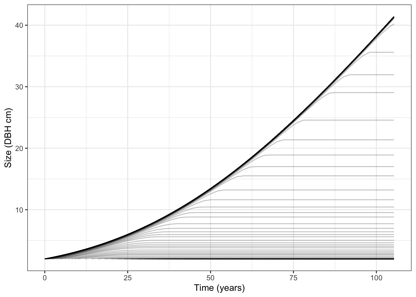
The run stops at around 105 years because that is the default max_patch_lifetime for K93 — the patch is still developing when it ends. Increasing the maximum patch lifetime extends the simulation to 700 years and allows the first cohorts to reach their maximum size of 136cm DBH, matching Fig. 2 of Kohyama (1993):
par$max_patch_lifetime <- 700
results <- run_scm(par, collect = TRUE)

tidy <- K93_expand_state(results)$species

ggplot(tidy, aes(time, height, group = node)) +
  geom_line(colour = util_colour_set_opacity("black", 0.25)) +
  labs(x = "Time (years)", y = "Size (DBH cm)") +
  theme_bw()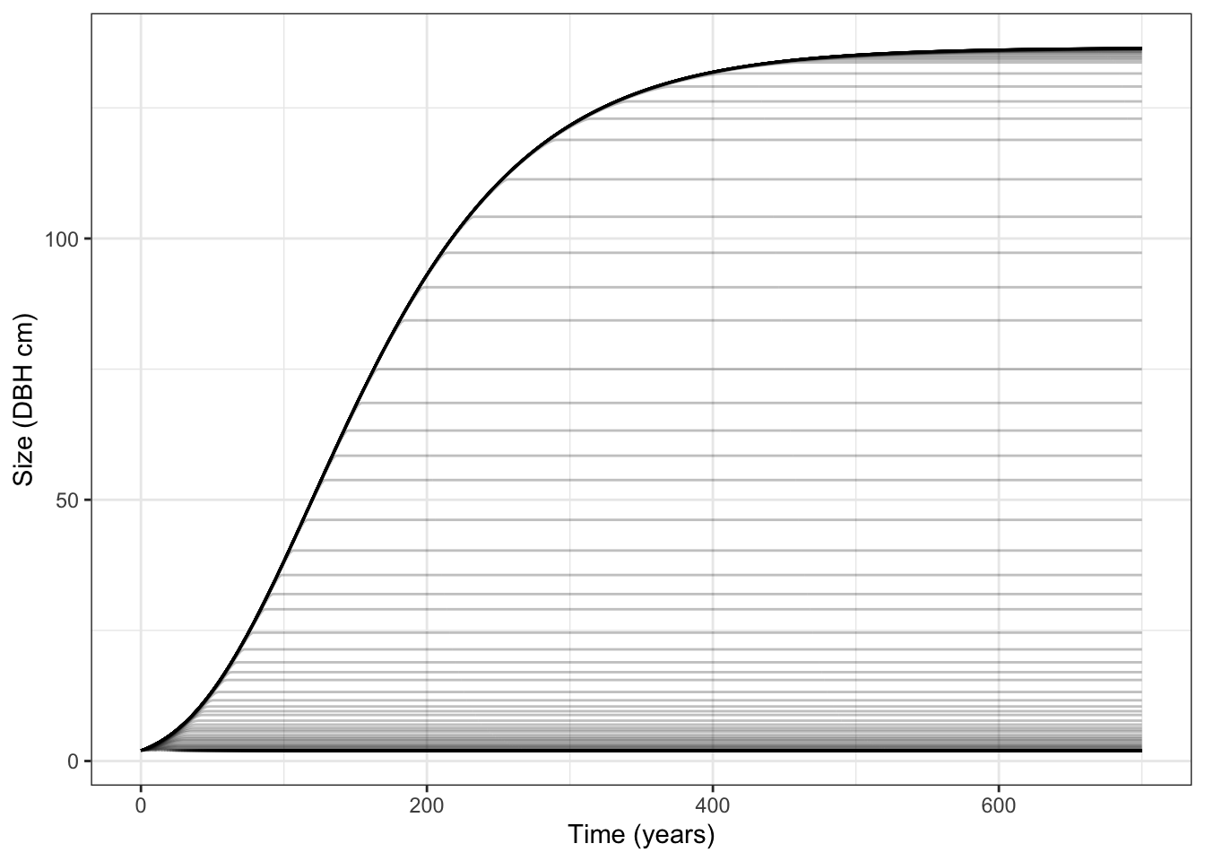
Note: we obtain more interesting results using the fast control parameters provided by the convenience function scm_base_parameters.
fast_par <- scm_base_parameters("K93")
fast_par$strategies[[1]] <- s
fast_par$max_patch_lifetime <- 700

results <- run_scm(fast_par, collect = TRUE)

tidy <- K93_expand_state(results)$species

ggplot(tidy, aes(time, height, group = node)) +
  geom_line(colour = util_colour_set_opacity("black", 0.25)) +
  labs(x = "Time (years)", y = "Size (DBH cm)") +
  theme_bw()
Weighting each cohort by its density shows how gap-formation can occur:
tidy %>%
  filter(density > 1e-7) %>%
  ggplot(aes(time, height, group = node, alpha = density)) +
  geom_line() +
  labs(x = "Time (years)",
       y = "Size (DBH cm)",
       alpha = "Density") +
  theme_bw()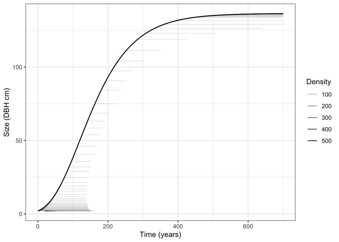
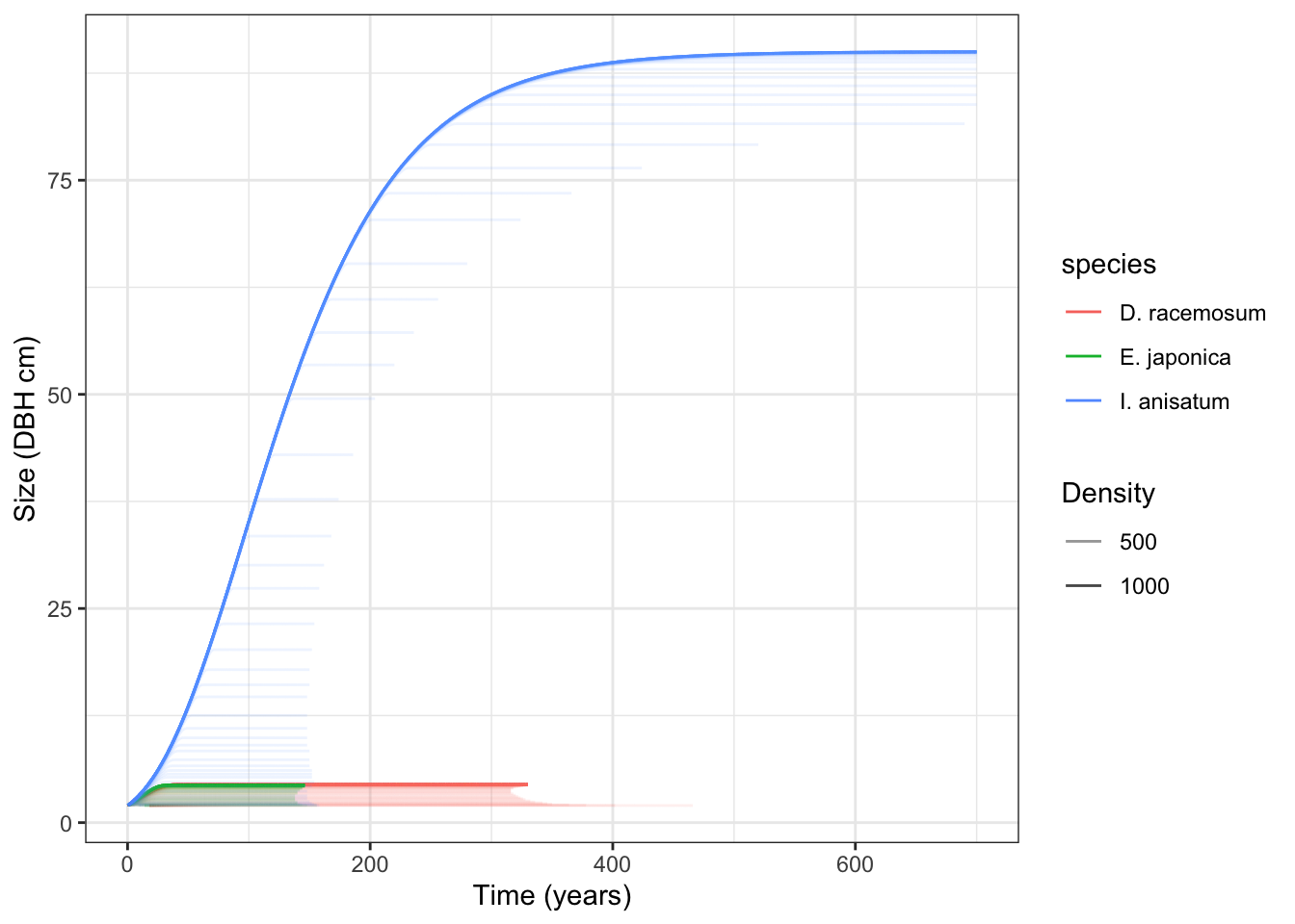
The Kohyama model also describes a patch with three species:
sp <- trait_matrix(c(0.042, 0.063, 0.052,
                     8.5e-3, 0.014, 0.015,
                     2.2e-4, 4.6e-4, 3e-4,
                     0.008, 0.008, 0.008,
                     1.8e-4, 4.4e-4, 5.1e-4,
                     1.4e-4, 2.5e-3, 8.8e-3,
                     0.044, 0.044, 0.044),
                   c("b_0", "b_1", "b_2",
                     "c_0", "c_1", "d_0", "d_1"))

fast_par2 <- scm_base_parameters("K93")
fast_par2$max_patch_lifetime <- 700
fast_par2$strategy_default$k_I <- 1e-6

sp_par <- expand_parameters(sp, fast_par2, birth_rate_list = rep(1, 3))

sp_results <- run_scm(sp_par, collect = TRUE)

sp_names <- c("D. racemosum", "I. anisatum", "E. japonica")

sp_tidy <- K93_expand_state(sp_results)$species %>%
  mutate(species = sp_names[as.integer(species)]) %>%
  filter(density > 1e-7)

ggplot(sp_tidy, aes(time, height, colour = species,
                    group = paste(species, node), alpha = density)) +
  geom_line() +
  labs(x = "Time (years)",
       y = "Size (DBH cm)",
       alpha = "Density") +
  theme_bw()