DD99: competition and evolutionary branching

How local competition can split one strategy into two

What the model represents

A single quantitative trait x, such as beak size, determines which part of a continuous resource an individual uses. The environment supports the largest population at an intermediate trait value x0, while individuals with similar trait values compete most strongly with one another.

These two effects can pull evolution in different directions. The resource distribution first draws the population towards x0. Once the population is there, however, strong competition among similar individuals can favour mutants on either side. The central strategy then becomes a fitness minimum and one lineage can split into two diverging strategies. This is evolutionary branching.

The model is based on Dieckmann and Doebeli (1999), On the origin of species by sympatric speciation.

Fitness equations

The model uses two Gaussian curves:

\[ K(x) = K_0 \exp\!\left(-\frac{(x-x_0)^2}{2\sigma_K^2}\right), \qquad C(d) = \exp\!\left(-\frac{d^2}{2\sigma_C^2}\right). \]

For a rare mutant y in a resident community \(\{x_i, N_i\}\) at demographic equilibrium, the invasion fitness (a per-capita growth rate, zero at the resident) is

\[ s(y) = r\left(1 - \frac{\sum_i N_i\, C(y - x_i)}{K(y)}\right). \]

A single resident reaches the equilibrium population size \(N^\* = K(x)\). The singular strategy is \(x^\* = x_0\). Its outcome depends on the widths of the two curves:

• if \(\sigma_C < \sigma_K\), competition acts over a narrower trait range than the resource distribution, and \(x_0\) is an evolutionary branching point;
• otherwise, \(x_0\) is an evolutionarily stable strategy (ESS).

Example analysis with regnans

library(regnans)

Choose parameters that produce branching (\(\sigma_C = 0.4 < \sigma_K = 1\)), then solve for the singular strategy:

h <- harness_dd99(r = 1, K0 = 500, x0 = 0, sigma_K = 1, sigma_C = 0.4)

out <- community_start(bounds(x = c(-2, 2)), harness = h) |>
  community_solve_singularity_1D()

as.numeric(out$traits)        # x* — expected 0 (= x0)

[1] 0

Finding the singular strategy does not tell us whether it is stable. We also check the curvature of invasion fitness at the resident. Positive curvature means the resident lies at a fitness minimum, so selection is disruptive and branching can occur:

resident_at <- function(h, x) {
  community_start(bounds(x = c(-2, 2)), harness = h) |>
    community_add(trait_matrix(x, "x")) |>
    community_demography()
}
curv <- function(comm, at, d = 1e-4) {
  f <- comm$fitness_function
  (f(at + d) - 2 * f(at) + f(at - d)) / d^2
}

curv(resident_at(h, 0), 0)                                   # > 0  → branching

[1] 5.25

curv(resident_at(harness_dd99(sigma_C = 1.5), 0), 0)        # < 0  → ESS

[1] -0.5555556

Pairwise invasibility plot

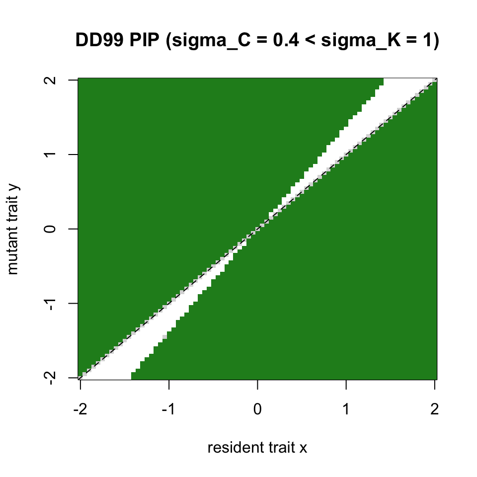
A pairwise invasibility plot shows the sign of \(s(y)\) for each resident x and mutant y. Green marks combinations for which the mutant can invade. The two green wedges on either side of x0 = 0 show that nearby mutants can invade the singular resident, which is the signature of branching.

xs <- seq(-2, 2, length.out = 81)
S <- sapply(xs, function(res) {
  resident_at(h, res)$fitness_function(xs)   # vector over all mutants
})                                            # S[mutant, resident]

image(xs, xs, t(sign(S)), col = c("white", "grey85", "forestgreen"),
      xlab = "resident trait x", ylab = "mutant trait y",
      main = "DD99 PIP (sigma_C = 0.4 < sigma_K = 1)")
abline(0, 1, lty = 2)