GM99: the evolution of seed size

Balancing seed number, survival, and competitive ability

What the model represents

Plants have a fixed amount of resource to invest in seeds. A plant can therefore produce many small seeds or fewer large ones. Large seeds are more likely to survive before competition and their seedlings compete more effectively, but each one is more expensive to make.

Seeds land at discrete safe sites, and the number arriving at any site is Poisson distributed. Seedlings at the same site then compete for its resources in a size-asymmetric lottery: larger seeds have an advantage. If that advantage is strong enough, the intermediate seed-size strategy becomes a branching point. Small, numerous seeds can then coexist with large, highly competitive seeds.

The model comes from Geritz, van der Meijden, and Metz (1999), Evolutionary Dynamics of Seed Size and Seedling Competitive Ability.

Fitness equations

Pre-competitive survival and competitive ability:

\[ s(x) = \max\!\left(0,\; 1 - 2e^{-\beta x}\right), \qquad c(x) = e^{\alpha x}. \]

A focal mutant x' lands in a site alongside \(k_j \sim \text{Poisson}(N_j)\) seedlings of each resident strategy x_j. Its expected share of the site, averaged across all possible seed arrivals, is

\[ g = \mathbb{E}\!\left[\frac{c(x')}{c(x') + \sum_j k_j\,c(x_j)}\right]. \]

Invasion fitness is the mutant’s expected number of established offspring (a lifetime reproductive ratio, = 1, i.e. log = 0, at equilibrium):

\[ W(x') = \frac{R}{x'}\, s(x')\, g . \]

A single resident reaches the density N* that solves \(\tfrac{R}{x}s(x)\,\tfrac{1-e^{-N}}{N} = 1\). Only the products \(\alpha R\) and \(\beta R\) affect the outcome. There is no formula for the singular strategy, so we find it numerically. Branching becomes more likely as the competitive asymmetry \(\alpha\) increases.

Example analysis with regnans

library(regnans)

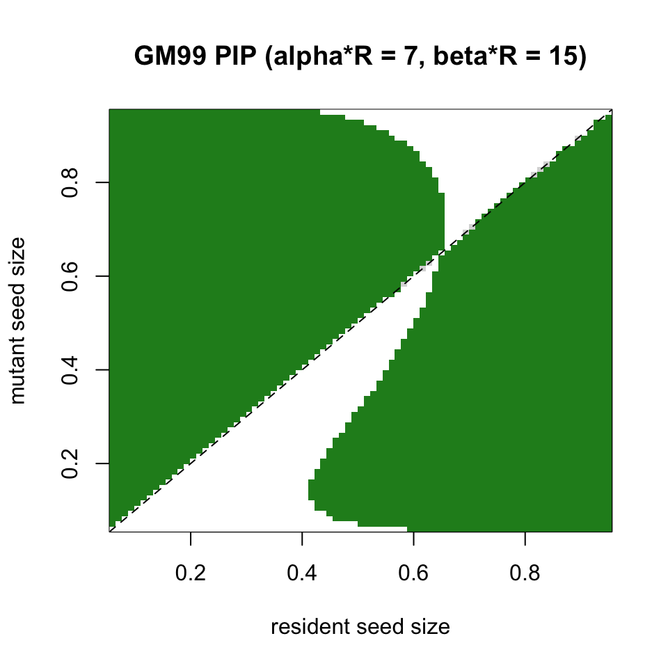
Hold pre-competitive survival at \(\beta R = 15\). Weak competitive asymmetry (\(\alpha R = 4.5\)) gives a single stable strategy, whereas stronger asymmetry (\(\alpha R = 7\)) gives a branching point.

solve_x <- function(alpha, beta = 15, bounds_x = c(0.06, 0.95)) {
  community_start(bounds(x = bounds_x),
                  harness = harness_gm99(alpha = alpha, beta = beta)) |>
    community_solve_singularity_1D()
}

css    <- solve_x(4.5)   # CSS
branch <- solve_x(7.0)   # branching point
c(css = as.numeric(css$traits), branch = as.numeric(branch$traits))

      css    branch 
0.1836584 0.6481792 

We classify each solution using the curvature of invasion fitness at the singular strategy. Negative curvature indicates a fitness maximum and a stable strategy; positive curvature indicates a fitness minimum and branching:

curv <- function(comm, at, d = 1e-4) {
  f <- comm$fitness_function
  (f(at + d) - 2 * f(at) + f(at - d)) / d^2
}
c(css = curv(css, as.numeric(css$traits)),
  branch = curv(branch, as.numeric(branch$traits)))

       css     branch 
-10.556158   1.439901 

As a check, a resident at its own demographic equilibrium must have a lifetime reproductive ratio of exactly 1, or a log fitness of 0:

comm <- community_start(bounds(x = c(0.06, 0.95)),
                        harness = harness_gm99(alpha = 7, beta = 15)) |>
  community_add(trait_matrix(0.645, "x")) |>
  community_demography()
comm$resident_fitness          # ≈ 0

[1] 0

Pairwise invasibility plot

The green regions show which mutant seed sizes can invade each resident seed size. The pattern around the singular strategy shows that mutants on either side can invade, as expected at a branching point.

h  <- harness_gm99(alpha = 7, beta = 15)
xs <- seq(0.06, 0.95, length.out = 81)
S <- sapply(xs, function(res) {
  community_start(bounds(x = range(xs)), harness = h) |>
    community_add(trait_matrix(res, "x")) |>
    community_demography() |>
    (\(comm) comm$fitness_function(xs))()
})
image(xs, xs, t(sign(S)), col = c("white", "grey85", "forestgreen"),
      xlab = "resident seed size", ylab = "mutant seed size",
      main = "GM99 PIP (alpha*R = 7, beta*R = 15)")
abline(0, 1, lty = 2)