library(plant)
library(regnans)
library(tidyverse)

model_support <- list(
  p = plant_default_assembly_pars(),
  plant_control = plant_default_assembly_control()
)Stochastic assembly
theory
This page runs stochastic community assembly with regnans and the full plant FF16 model. The maximum-fitness method always adds the mutant with the highest invasion fitness. Stochastic assembly instead draws a new mutant at random from a Gaussian mutation distribution, controlled by vcv.
The sequence of mutants therefore resembles a noisy evolutionary walk rather than a direct climb towards the highest-fitness strategy. The first example allows leaf mass per area (lma) to vary. The second allows both lma and height at maturation (hmat) to vary.
Leaf mass per area (lma)
Assembly
control <- assembler_control(
  list(
    run_type = "single_step",
    birth_type = "stochastic",
    vcv = diag(1)
  )
)

community0 <- community_start(bounds(lma = c(0.01, 1)), model_support = model_support)
obj <- assembler_run(assembler_start(community0, control = control), nsteps = 60)

obj$community$traits
lma
[1,] 0.31224478
[2,] 0.09486322
[3,] 0.30855811obj$community$birth_rate[1] 0.443440488 4.652990951 0.004294305The assembly walk
tidy_assembly() gives one row for each resident strategy at each step. After unnesting the trait values, we can plot how the community changes through time. Larger points represent strategies with higher birth rates:
tidy_assembly(obj) |>
  filter(resident) |>
  unnest(traits) |>
  mutate(step = as.integer(step)) |>
  ggplot(aes(step, lma, size = births)) +
  geom_point(alpha = 0.4, colour = "forestgreen") +
  scale_y_log10() +
  labs(x = "assembly step", y = "lma", size = "birth rate") +
  theme_classic()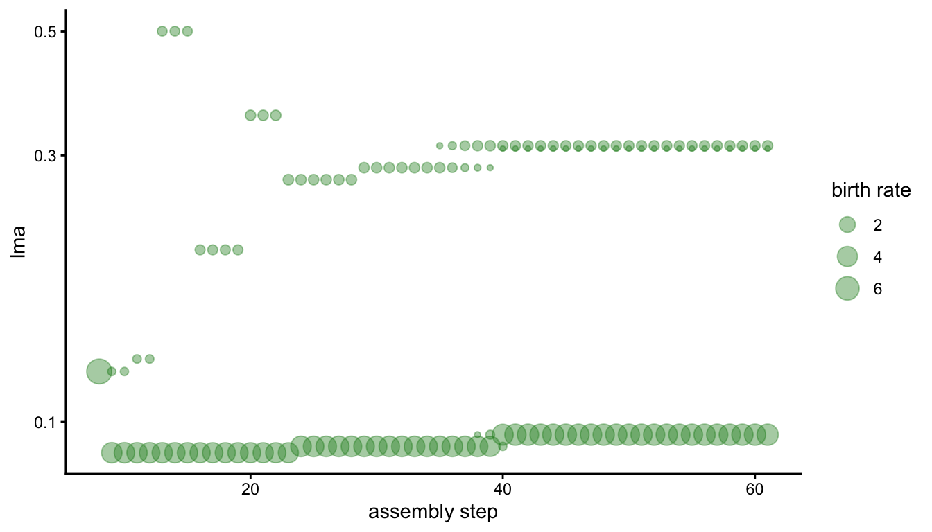
Fitness landscape
Stochastic runs do not calculate a complete fitness landscape by default. We can evaluate it on a grid for the final community. Resident strategies are marked in red; they should lie at or near zero fitness, with no large positive invasion peaks remaining:
obj$community <- community_fitness_landscape(obj$community, method = "grid", n_evals = 100)
fp <- obj$community$fitness_points
ggplot(fp, aes(lma, fitness)) +
  geom_line() +
  geom_hline(yintercept = 0, linetype = "dashed") +
  geom_point(data = filter(fp, resident), colour = "red", size = 2) +
  scale_x_log10() +
  theme_classic()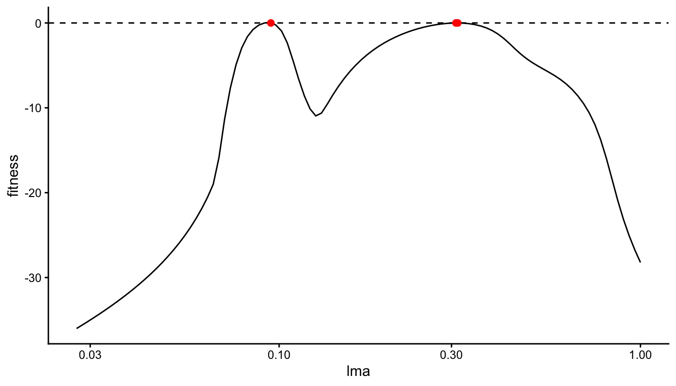
Leaf mass per area and height at maturation
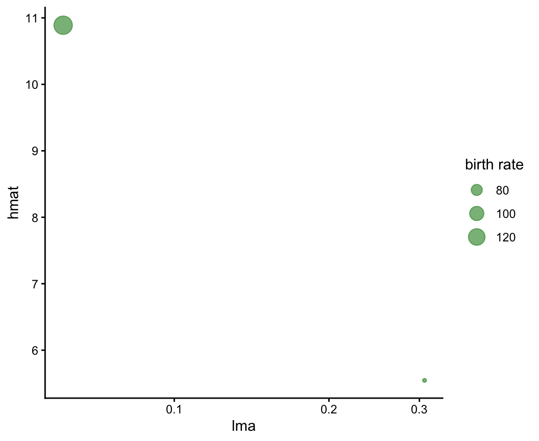
With a two-dimensional mutation distribution, both lma and hmat can change at each step. The community is then assembled across a two-dimensional trait space.
control2 <- assembler_control(
  list(
    run_type = "single_step",
    birth_type = "stochastic",
    compute_viable_fitness = FALSE,
    vcv = diag(2)
  )
)

community0 <- community_start(bounds(lma = c(0.01, 1), hmat = c(0.5, 30)),
                             model_support = model_support)
obj2 <- assembler_run(assembler_start(community0, control = control2), nsteps = 10)

obj2$community$traits
lma hmat
[1,] 0.06078574 10.889714
[2,] 0.30697190 5.545609obj2$community$birth_rate[1] 137.56505 61.09276The final plot shows the assembled strategies in the lma-hmat trait space. Larger points represent strategies with higher birth rates:
as_tibble(obj2$community$traits) |>
  mutate(birth_rate = obj2$community$birth_rate) |>
  ggplot(aes(lma, hmat, size = birth_rate)) +
  geom_point(colour = "forestgreen", alpha = 0.6) +
  scale_x_log10() +
  labs(size = "birth rate") +
  theme_classic()