library(plant)
library(parallel)
ncores <- detectCores() - 1
p0 <- scm_base_parameters("FF16")
p <- add_strategies(p0, trait_matrix(0.0825, "lma"), birth_rate = 20)
times_default <- p$node_schedule_times[[1]]The node-spacing algorithm
implementation
NotePrerequisites
This page builds on The size-structured PDE and the method of characteristics. Read those first if the notation here is unfamiliar.
The idea first
plant never tracks a continuous size distribution directly. Instead it approximates that distribution with a finite collection of cohorts, each one a single representative individual standing in for all the plants born at roughly the same moment. As those cohorts grow and thin over time, the model has to decide two things: when to add a new cohort to the population, and how to space the existing ones so the whole collection still traces out the size distribution faithfully.
This is a genuine trade-off. Add too few cohorts, or space them too coarsely, and the model smooths over real structure in the population, missing the sharp features that matter for growth and competition. Add too many, or space them too finely, and the simulation grinds through far more bookkeeping than the answer warrants, most of it spent refining regions that were already accurate enough. The art of the node-spacing algorithm is finding, at every point in a patch’s development, the smallest set of cohorts that keeps the approximation error below a chosen tolerance, and no smaller.
The rest of this page makes this precise.
Background
As described in the size-structured PDE page, the spacing of nodes can affect the accuracy of integration over the size-density distribution. plant uses an adaptive algorithm to build an appropriately spaced node schedule with the desired accuracy at every time point, using as few nodes as possible.
The refinement algorithm takes an initial vector of introduction times and considers, for each node, whether removing that node causes the error introduced when integrating two specified functions over the size-density distribution to jump over the allowable error threshold schedule_eps. This calculation is repeated for every time step in the development of the patch. A new node is introduced immediately prior to any node failing these tests. The dynamics of the patch are then simulated again and the process is repeated, until all integrations at all time points have an error below the tolerable limit schedule_eps. Decreasing schedule_eps demands higher accuracy from the solver, and thus increases the number of nodes being introduced. Note that we are assessing whether removing an existing node causes the error to jump above the threshold limit, and using this to decide whether an extra node – in addition to the one used in the test – should be introduced. Thus, the actual error is likely to be lower than, but at most equal to, schedule_eps.
This refinement now lives entirely in C++, inside the SCM solver. You trigger it from R with:
scm <- run_scm(p, refine_schedule = TRUE)
p_refined <- scm$parameters
run_scm(refine_schedule = TRUE) calls SCM::refine_schedule(), which runs the solver, collects the per-node integration error as the patch develops, splits the flagged intervals, and repeats. The refined schedule and the ODE times of the final run are written back into the returned parameters, so the Parameters object remains self-describing. (Earlier versions of plant did this work in R via the build_schedule() and run_scm_error() functions; both have been removed in favour of the in-solver implementation.)
This page shows some details of node splitting, most of which happens automatically. It’s probably not very interesting to most people, only those interested in knowing how the SCM technique works in detail. It also uses a lot of non-exported, non-documented functions from plant so you’ll see a lot of plant::: prefixes.
Node introduction times
The default node introduction times are designed to concentrate node introductions onto earlier times, based on empirical patterns of node refining:
plot(times_default, cex=.2, pch=19, ylab="Time (years)", las=1)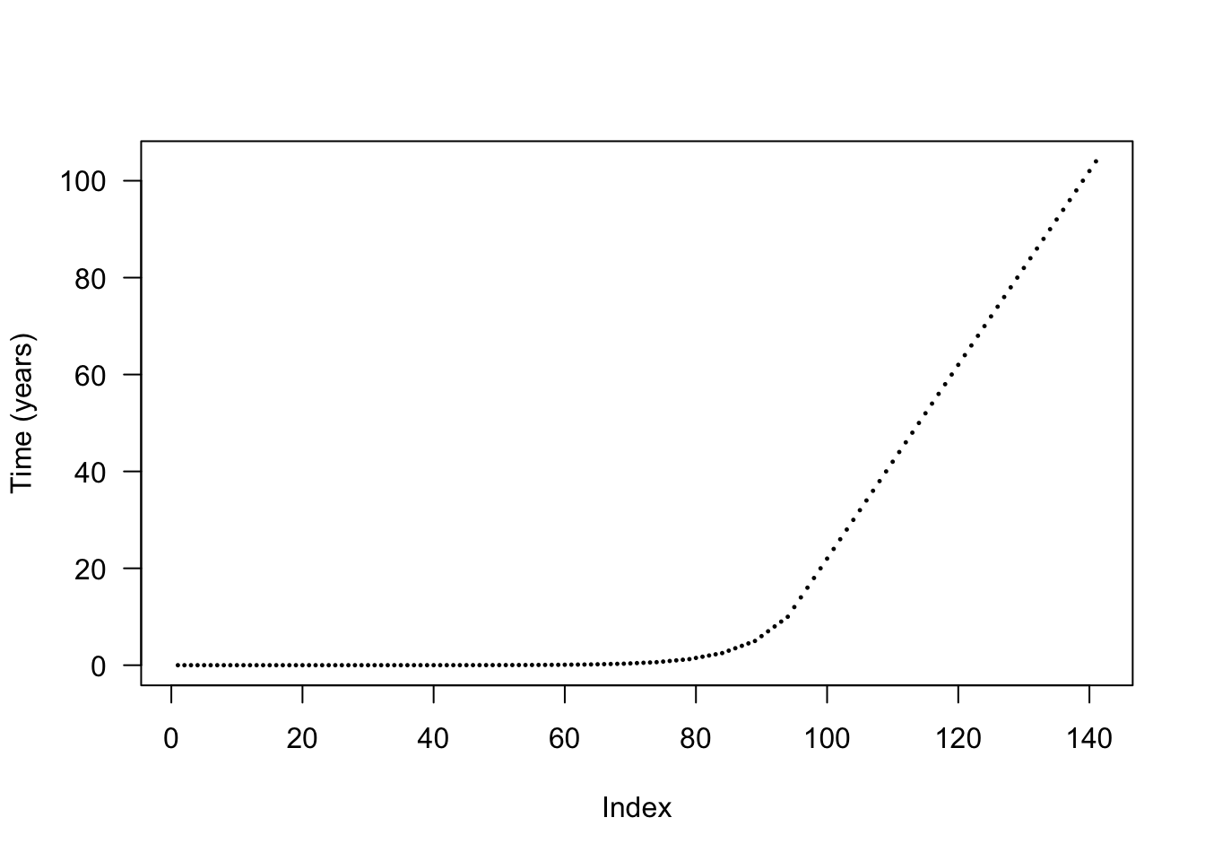
The actual differences are stepped in order to increase the chance that nodes from different species will be introduced at the same time and reduce the total amount of work being done.
plot(diff(times_default), pch=19, cex=.2, ylab="Time difference (years)", las=1)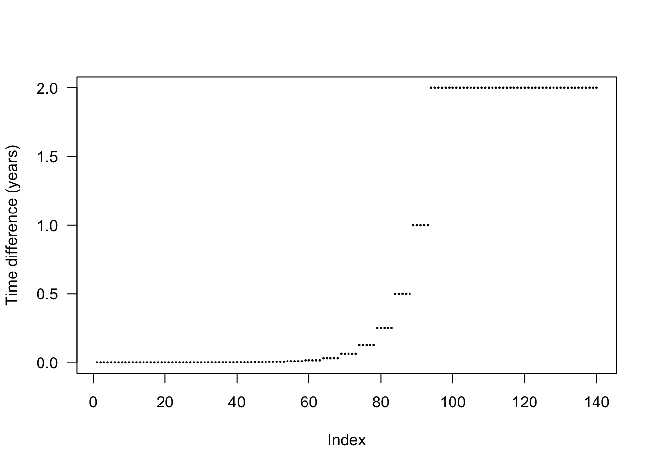
Estimating error in node spacing
We can assess the impact of node spacing on integration error by examining the cumulative offspring production of a patch.
Increasing the number of nodes is expected to increase integration accuracy at the expense of more computational effort. We can create more refined schedules by interleaving points into the existing schedule:
interleave <- function(x) {
  n <- length(x)
  xp <- c(x[-n] + diff(x) / 2, NA)
  c(rbind(x, xp))[- 2 * n]
}


times_2x <- interleave(times_default)
times_4x <- interleave(times_2x)

plot(times_default, xlab = "Node #", ylab="Time (years)",
     xlim = c(1, length(times_4x)), las=1, pch = 19, cex=.2,)
points(times_2x, pch=19, cex=.2, las=1, col = "blue")
points(times_4x, pch=19, cex=.2, las=1, col = "red")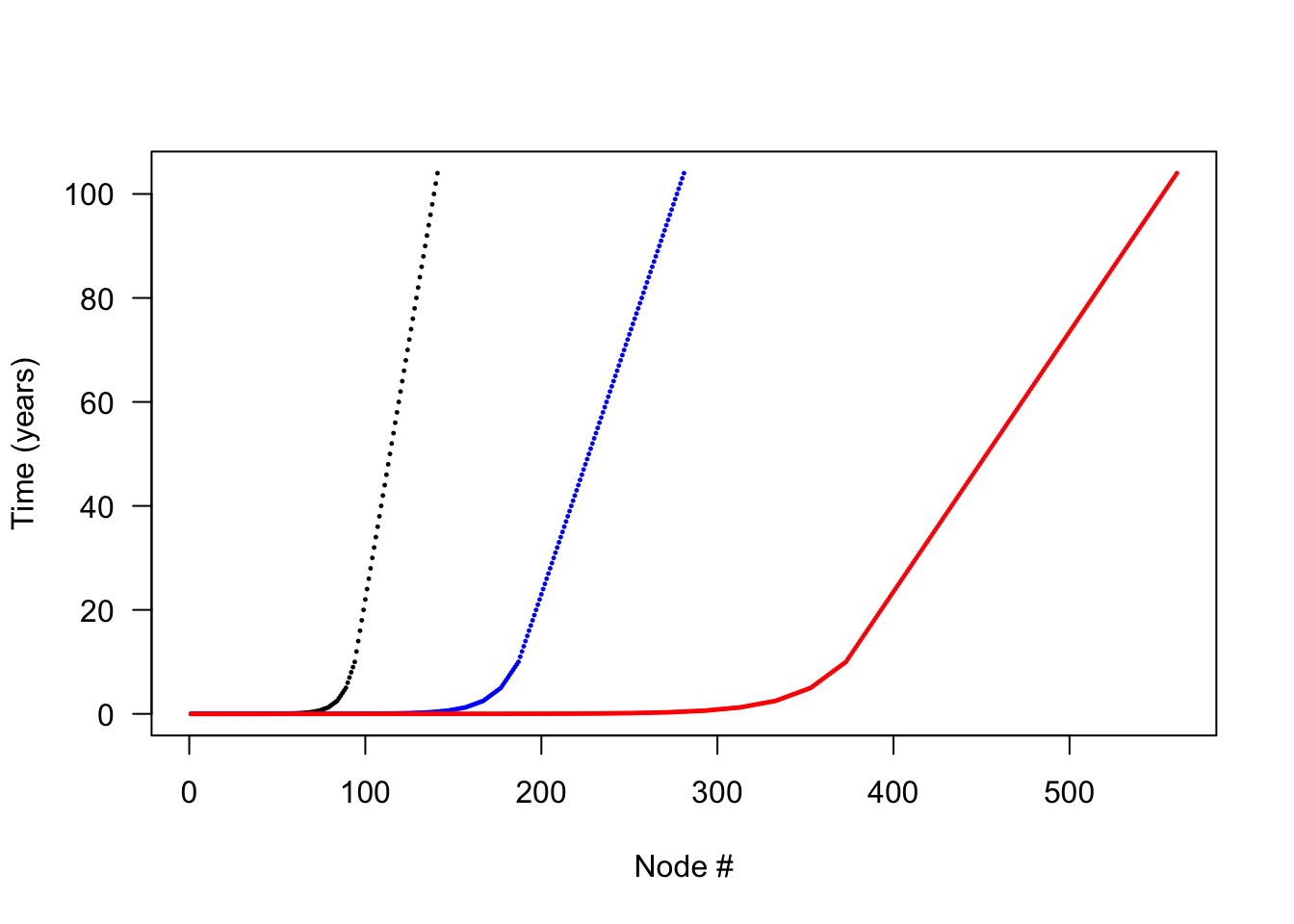
Each schedule runs for the same duration, but times_4x has 4x as many nodes. Running a patch with each node schedule allows us to compare the propagule outputs:
run_with_times <- function(p, t) {
  p$node_schedule_times[[1]] <- t

  start <- Sys.time()
  offspring_production <- run_scm(p)$offspring_production
  print(paste("Time to solve:", round(Sys.time() - start, 2)))

  return(offspring_production)
}

offspring_production_default <- run_with_times(p, times_default)
[1] "Time to solve: 0.15"offspring_production_2x <- run_with_times(p, times_2x)[1] "Time to solve: 0.27"offspring_production_4x <- run_with_times(p, times_4x)[1] "Time to solve: 0.83"node_range <- c(length(times_default), length(times_2x),
length(times_4x))
offspring_production_range <- c(offspring_production_default, offspring_production_2x,
offspring_production_4x)Quadrupling the number of nodes results in nearly a 6x increase in runtime, eight times the nodes takes roughly 26x longer (the latter not shown).
plot(x = node_range, y = offspring_production_range,
     xlab="Number of node introductions", ylab="Offspring production", las=1)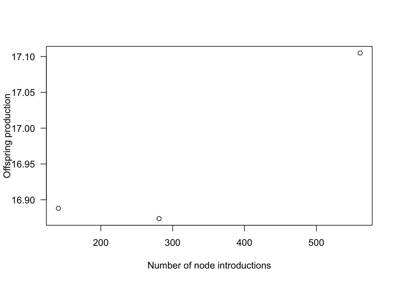
Offspring production increases as nodes are introduced more finely, though at a saturating rate, meaning there are diminishing returns in accuracy for additional nodes.
The differences in offspring production are not actually that striking (perhaps 1%) but the introduced variation creates instabilities of sufficient concern.
Individual offspring production contributions
Where is the fitness difference driving change in offspring production coming from?
Consider adding a single additional node at one of the points along the first vector of times times_default and computing the output offspring production:
The next chunk runs the solver once per insertion position in parallel via mclapply. It is a heavy computation, so we mark it #| eval: false and show the pre-rendered figure below; the helper definitions are retained for reference.
insert_time <- function(i, x) {
  j <- seq_len(i)
  c(x[j], (x[i] + x[i+1])/2, x[-j])
}
run_with_insert <- function(i, p, t) {
  run_with_times(p, insert_time(i, t))
}

insert_positions <- seq_len(length(times_default) - 1)
offspring_productions <- unlist(mclapply(insert_positions, run_with_insert,
                              p, times_default, mc.cores = ncores))

offspring_production_differences <- offspring_productions - offspring_production_default

plot(insert_positions, offspring_production_differences,
     xlab="Node #", ylab="Difference from default Offspring production", las=1)
abline(h=0, col="grey")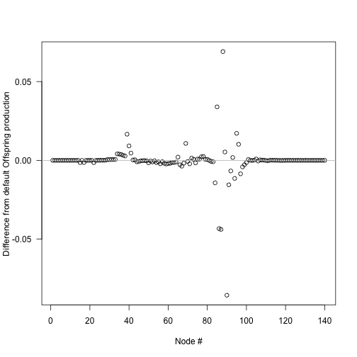
The biggest deviations in output offspring production come about half way through the schedule, though because of the compression of early times this occurs fairly early in patch development:
The next chunk just replots the differences computed above against time, so it is also marked #| eval: false and shown as a pre-rendered figure.
times_interpolated <- (times_default[-1L] +
                         times_default[-length(times_default)]) / 2

plot(times_interpolated, offspring_production_differences,
     xlab="Time (years)", ylab="Difference from default Offspring production", las=1)
abline(h=0, col="grey")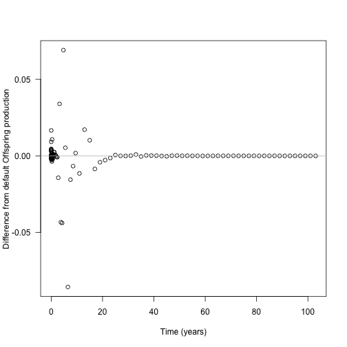
Now look at the contribution of different nodes to the overall patch output (log scaled for clarity).
Each node carries its own lifetime offspring production, accumulated inside the ODE and exposed per node via the species’ net_reproduction_ratio_by_node. (This is the unweighted per-node contribution; the SCM weights these by the patch-age density and survival during dispersal when integrating overall fitness.)
This chunk depends on times_interpolated, top_5 and offspring_production_differences produced by the parallel chunks above, so it is shown as a pre-rendered figure rather than executed.
default <- run_scm(p)

contributions <- default$patch$species[[1]]$net_reproduction_ratio_by_node

top_5 <- order(abs(offspring_production_differences), decreasing=TRUE)[1:5]

# drop the first node (zero contribution) to avoid log(0)
keep <- contributions > 0
plot(times_default[keep], contributions[keep], log = "y",
     xlab="Time (years)", ylab="Offspring production (log scale)", las=1)
abline(v=times_interpolated[top_5], col=c("red", rep("grey", 4)))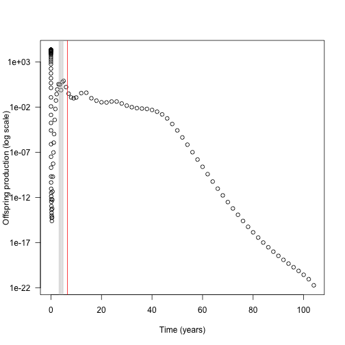
In this case almost all the contribution comes from early nodes (this is essentially a single-age stand of pioneers).
Overlaid on this are the five nodes where extra refinement (i.e. inserting an additional node) causes the largest change in overall offspring production output (biggest difference in red).
The difference is not coming from offspring production contributions of those nodes, which is basically zero, though it is higher than the surrounding nodes.
Individual competitive impacts
If the inserted nodes are not altering offspring production through individual contributions, they may be altering the output of neighbouring nodes through competitive interactions.
Here we investigate the differences in patch light environment after introducing the single node driving the greatest difference in seed output identified above.
First we run patches with and without the extra node, collecting the complete set of patch conditions at each timestep with run_scm(collect = TRUE).
This chunk depends on top_5 and insert_time() from the parallel analysis above, so it is shown but not executed.
collect_with_times <- function(p, t) {
  p$node_schedule_times[[1]] <- t
  result <- run_scm(p, collect = TRUE)
  return(result)
}

insert_position <- top_5[1]
times_insert <- insert_time(insert_position, times_default)

results_default <- collect_with_times(p, times_default)
results_insert <- collect_with_times(p, times_insert)
In order to make a direct comparison, we need to interpolate the light environment over a common set of heights at each time step.
We reconstruct the light environment spline for both runs, and compute light_availability in both:
interpolated_light_availability <- function(env, heights) {
  # intialise new spline with existing values
  spline <- plant:::Interpolator()
  spline$init(env[, 1], env[, 2])

  # subset to valid heights in patch
  patch_heights <- heights < spline$max

  # evaluate over list of heights and zero
  y <- spline$eval(heights)
  y[!patch_heights] = 0

  return(y)
}

n = length(results_default$time)

max_height <- max(results_default$env[[n]][, 1],
                  results_insert$env[[n+1]][, 1])

heights <- seq(0, max_height, length.out=201)
light_availability_spline_default <- sapply(results_default$env, interpolated_light_availability, heights)
light_availability_spline_insert <- sapply(results_insert$env, interpolated_light_availability, heights)

light_availability_spline_difference <- t(light_availability_spline_insert[, -(insert_position + 1)] - canopy_default)
light_availability_spline_difference[abs(light_availability_spline_difference) < 1e-10] <- NA
Taking the difference between light environments at each height and timestep, the resulting image plot is blue in regions where the refined light environment, with the additional node is lighter (higher light_availability) and red in regions where the the light environment is darker with the additional node.
This image plot depends on the snapshots collected above, so it is shown but not executed. (The source did not pre-render this figure.)
# ColorBrewer's RdBu palette
cols <- c("#B2182B", "#D6604D", "#F4A582", "#FDDBC7",
          "#D1E5F0", "#92C5DE", "#4393C3", "#2166AC")
pal <- colorRampPalette(cols)(20)

image(results_default$time, heights, light_availability_spline_difference,
      xlab="Time (years)", ylab="Height (m)", las=1, col=pal)
Shading is lower for ~7 m tall nodes at year 25. This increased competitive intensity may be driving differences in offspring production.
Monitoring integration accuracy
The SCM monitors two integrations over the size-density distribution as the patch develops and uses the larger of the two errors to decide where to refine:
- a competition (leaf-area) error, measuring how much removing a node changes the estimate of total leaf area in the patch; and
- an offspring-production error, measuring how much removing a node changes the estimate of total seed production from the patch.
The relative error of each integration is computed with the local_error_integration function. The competition error is sampled at every introduction step as the patch develops, while the offspring-production error is computed once at the end of the run. Both are now accumulated inside SCM::run() when error collection is enabled, and the per-node maximum of the two is exposed as refinement_error_by_node – the signal that drives refinement:
scm <- run_scm(p)            # SCM object
scm$collect_refinement_errors <- TRUE
scm$run()                    # rerun, now accumulating the error signal

combined <- scm$refinement_error_by_node[[1]]

plot(times_default, combined, type = "h",
     xlab = "Introduction time (years)", ylab = "Combined per-node error", las = 1)
abline(h = Control()$schedule_eps, col = "red", lty = 2)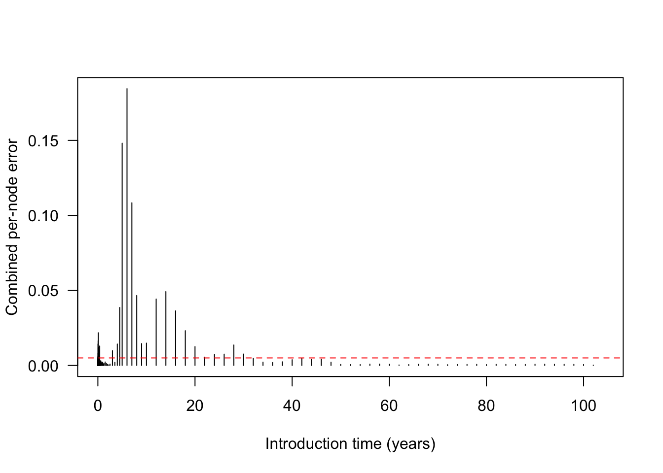
Nodes whose combined error exceeds the threshold schedule_eps (red line) are the ones the refinement step will split.
To see how the competition error builds up over the development of the patch we can reconstruct the per-step matrix that the solver accumulates internally. We run the SCM once collecting a patch snapshot after each introduction, then recompute the competition error from each snapshot. Each row is one introduction step; each column is a node:
competition_error_matrix <- function(p, env = NULL, ctrl = Control()) {
  scm <- run_scm(p, env, ctrl)   # build + run, returns the SCM object
  scm$reset()                    # rewind so we can re-run while collecting
  scm$collect <- TRUE
  scm$run()

  ## history[[1]] is the initial (empty) patch; the rest are the state after
  ## each introduction. Recompute species 1's per-node competition error.
  rows <- lapply(scm$history[-1], function(h)
    h$species[[1]]$compute_competition_effect_by_nodes_error(h$compute_competition(0)))
  ncol <- max(lengths(rows))
  do.call(rbind, lapply(rows, function(r) c(r, rep(NA, ncol - length(r)))))
}

patch_error_lai <- competition_error_matrix(p)
image(times_default, times_default, patch_error_lai,
      xlab="Patch age (years)", ylab="Introduction time (years)", las=1)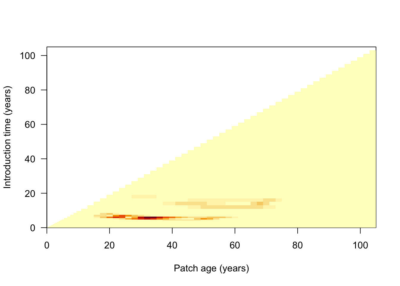
SCM::refine_schedule() uses exactly this combined error to find an appropriately refined node spacing that minimises both integration errors.
scm_refined <- run_scm(p, refine_schedule = TRUE)
p_refined <- scm_refined$parameters
offspring_production_refined <- scm_refined$offspring_production
We can see the impact of this refinement by repeating our earlier analysis – inserting a new node at each timestep and extracting the offspring production – this time plotting on the same vertical scale as the unrefined run above:
This final analysis again runs the solver once per insertion position via mclapply (and depends on offspring_production_differences from the earlier parallel run), so it is marked #| eval: false and shown as a pre-rendered figure.
times_refined <- p_refined$node_schedule_times[[1]]

insert_positions <- seq_len(length(times_refined) - 1)

offspring_productions_refined <- unlist(mclapply(insert_positions, run_with_insert,
                                      p_refined, times_refined,
                                      mc.cores = ncores))

refined_differences <- offspring_productions_refined - offspring_production_refined

plot(insert_positions, refined_differences,
     xlab = "Index", ylab = "Offspring production differences", las = 1,
     ylim = range(offspring_production_differences))
abline(h = 0, col = "grey")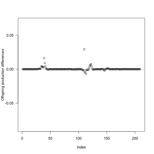
On this common scale it is clear that refinement noticeably shrinks the variation introduced by inserting an extra node. In relative terms the largest remaining change is only 0.0017. The refined node introduction schedule reaches an offspring production near the saturating value identified above, but with 210 nodes rather than the 561 nodes used in naive interpolation.