GK98: adaptation across different habitats

How soft selection can maintain two strategies

What the model represents

This model follows one trait across several habitats, each with a different optimal trait value. Selection within each habitat favours individuals close to its local optimum. Density regulation is soft: every habitat contributes a fixed share of the next generation, regardless of how many individuals survive there. This prevents the most productive habitat from dominating the whole population.

When habitat optima are close together, evolution settles on one compromise strategy. When they are far enough apart, the same compromise attracts gradual evolution but can be invaded after it is reached. The population then branches into two strategies adapted to different parts of the habitat distribution.

The model comes from Geritz et al. (1998), Evolutionarily singular strategies and the adaptive growth and branching of the evolutionary tree (Geritz, Kisdi, Meszéna, & Metz, 1998).

Fitness equations

There are three habitats (\(m=3\)), with optima \(\mu = (-d, 0, d)\). Habitat \(j\) has capacity \(K_j\) and therefore contributes the fraction \(c_j = K_j/\sum_h K_h\) of the next generation. Survival within each habitat is a Gaussian curve with width \(\sigma\):

\[ f_j(x) = \exp\!\left(-\frac{(x-\mu_j)^2}{2\sigma^2}\right). \]

For a single resident x, the invasion fitness of a mutant y (a log per-capita growth, zero at the resident) is

\[ s_x(y) = \log \sum_{j} c_j \, \frac{f_j(y)}{f_j(x)}. \]

The singular strategy is the capacity-weighted mean optimum, \(x^\* = \sum_j c_j \mu_j\). It equals zero when the three habitats have equal capacities. Evolution always moves towards this strategy, but what happens on arrival depends on the separation of habitat optima:

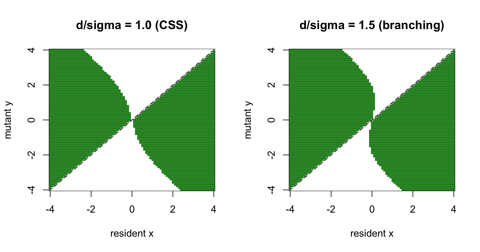
• if \(d/\sigma > \sqrt{3/2} \approx 1.2247\), it is a branching point;
• below that threshold, it is a continuously stable strategy (CSS): evolution approaches it and nearby mutants cannot invade it.

Example analysis with regnans

library(regnans)

h <- harness_gk98(d = 1.5, sigma = 1)   # d/sigma = 1.5 > sqrt(1.5) → branching

out <- community_start(bounds(x = c(-4, 4)), harness = h) |>
  community_solve_singularity_1D()

as.numeric(out$traits)   # x* — expected 0 (symmetric three-patch)

[1] -6.927792e-14

We can recover the branching threshold numerically. The following code finds where the curvature of invasion fitness at x* = 0 changes sign:

curv0 <- function(d, sigma = 1, h = 1e-4) {
  comm <- community_start(bounds(x = c(-4, 4)),
                          harness = harness_gk98(d = d, sigma = sigma)) |>
    community_add(trait_matrix(0, "x")) |>
    community_demography()
  f <- comm$fitness_function
  (f(h) - 2 * f(0) + f(-h)) / h^2
}

uniroot(curv0, c(1.0, 1.5))$root   # ≈ sqrt(3/2)

[1] 1.22474

sqrt(3 / 2)

[1] 1.224745

Pairwise invasibility plots either side of the threshold

The left plot uses closely spaced habitat optima and has one stable strategy. The right plot uses more widely spaced optima and shows the invasion pattern around a branching point.

pip <- function(h, xs) {
  sapply(xs, function(res) {
    community_start(bounds(x = range(xs)), harness = h) |>
      community_add(trait_matrix(res, "x")) |>
      community_demography() |>
      (\(comm) comm$fitness_function(xs))()
  })
}
xs <- seq(-4, 4, length.out = 81)

op <- par(mfrow = c(1, 2))
for (d in c(1.0, 1.5)) {
  S <- pip(harness_gk98(d = d, sigma = 1), xs)
  image(xs, xs, t(sign(S)), col = c("white", "grey85", "forestgreen"),
        xlab = "resident x", ylab = "mutant y",
        main = sprintf("d/sigma = %.1f (%s)", d,
                       if (d > sqrt(1.5)) "branching" else "CSS"))
  abline(0, 1, lty = 2)
}

par(op)

References

Geritz, S. A. H., Kisdi, É., Meszéna, G., & Metz, J. A. J. (1998). Evolutionarily singular strategies and the adaptive growth and branching of the evolutionary tree. Evolutionary Ecology, 12(1), 35–57. doi:10.1023/A:1006554906681