library(regnans)Community assembly with simple models
From one successful mutant to a community of coexisting strategies
A pairwise invasibility plot (PIP) asks whether one mutant can invade a community containing one resident strategy. Community assembly goes further by allowing several resident strategies to coexist.
At each assembly step, the algorithm:
- finds the mutant with the highest invasion fitness;
- adds that mutant to the resident community;
- returns the community to demographic equilibrium; and
- removes any resident strategies whose populations fall to zero.
Repeating these steps shows how evolutionary branching and competition can build a multi-strategy community. The small models in regnans make this process quick enough to explore interactively.
A note on trait scale
The assembly algorithm must search across possible trait values. The scale used for that search matters:
- use a log scale for strictly positive traits, such as
plant’s leaf mass per area (lma) or seed size in GM99; - use a linear scale for traits that can be zero or negative, as in DD99 and GK98.
Set the scale with community_start(trait_scale = ...). The default is "log".
DD99 — limiting similarity in one dimension
When competition covers a narrower trait range than the resource distribution (sigma_C < sigma_K), the resource optimum is a branching point. Repeated branching fills trait space with coexisting strategies. Strategies that are too similar compete too strongly to coexist, so the survivors are spaced apart. This spacing is called limiting similarity.
h <- harness_dd99(x0 = 0, sigma_K = 1, sigma_C = 0.4)
comm <- community_start(bounds(x = c(-3, 3)), harness = h, trait_scale = "linear",
                        fitness_control = list(method = "grid", n_evals = 150))
a <- assembler_start(comm, assembler_control(list(birth_type = "maximum")))
a <- assembler_run(a, 14)

cat(length(a$community), "coexisting species\n")
11 coexisting speciesxs <- sort(as.numeric(a$community$traits))
plot(xs, rep(1, length(xs)), pch = 19, col = "forestgreen", yaxt = "n",
ylab = "", xlab = "trait x", xlim = c(-3, 3),
main = sprintf("DD99 assembly: %d species (limiting similarity)", length(xs)))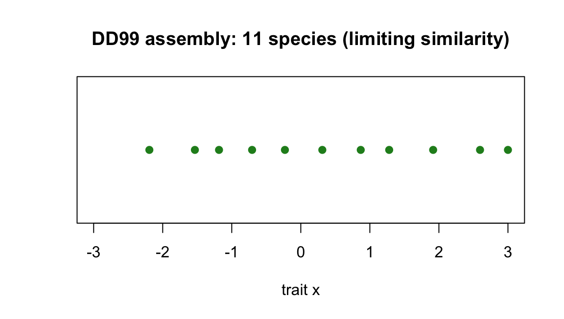
GK98 — branching to a protected dimorphism
Soft selection keeps the model’s total population fixed, so an empty community cannot be colonised in the usual way. We instead seed the community with one strategy and allow it to evolve. At d/sigma = 1.5, which is above the branching threshold \(\sqrt{3/2}\), the original strategy splits into two coexisting strategies. This stable pair is called a protected dimorphism.
comm <- community_start(bounds(x = c(-4, 4)), harness = harness_gk98(d = 1.5, sigma = 1),
                        trait_scale = "linear",
                        fitness_control = list(method = "grid", n_evals = 150))
a <- assembler_start(comm, assembler_control(list(birth_type = "maximum")))
a <- assembler_set_traits(a, trait_matrix(0, "x"))   # seed the first type
a <- assembler_run(a, 10)

sort(round(as.numeric(a$community$traits), 3))        # a symmetric dimorphism
[1] -0.828 0.874GM99 — a seed-size polymorphism
Strong size-asymmetric competition (alpha*R = 7) drives branching in seed size. Starting from an empty community produces a mixture of small- and large-seeded strategies. GM99 evaluates a multidimensional Poisson sum when several residents are present, so this example is slower than the other simple models. Assembling even a few strategies can take several seconds.
comm <- community_start(bounds(x = c(0.06, 0.95)), harness = harness_gm99(alpha = 7, beta = 15),
                        fitness_control = list(method = "grid", n_evals = 80))
a <- assembler_start(comm, assembler_control(list(birth_type = "maximum")))
a <- assembler_run(a, 4)
sort(round(as.numeric(a$community$traits), 3))   # e.g. 0.11, 0.45, 0.69 — small, medium, large seeds
DD99 in two trait dimensions
harness_dd99_nd() extends DD99 to more than one trait. The resource and competition curves are products of separate Gaussian curves for each trait, so every trait has its own optimum and curve widths. The joint singular strategy is x* = x0. Evolution branches along any trait for which sigma_C < sigma_K.
The same assembler_run() function handles two-dimensional assembly. We only need to provide bounds for two traits and use the multi-trait harness:
h2 <- harness_dd99_nd(x0 = c(0, 0), sigma_K = c(1, 1), sigma_C = c(0.5, 0.5))
comm <- community_start(bounds(x1 = c(-3, 3), x2 = c(-3, 3)), harness = h2,
                        trait_scale = "linear",
                        fitness_control = list(method = "grid", n_evals = 40))
a <- assembler_start(comm, assembler_control(list(birth_type = "maximum")))
a <- assembler_run(a, 40)

cat(length(a$community), "coexisting species in 2D\n")
27 coexisting species in 2Dplot(a$community$traits[, 1], a$community$traits[, 2], pch = 19, col = "forestgreen",
xlab = "trait x1", ylab = "trait x2", xlim = c(-3, 3), ylim = c(-3, 3),
main = sprintf("DD99 2D assembly: %d species", length(a$community)))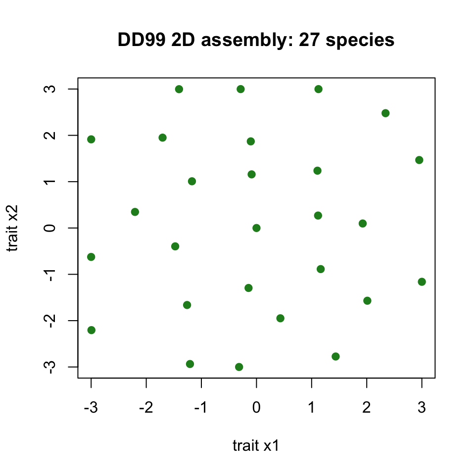
The resulting strategies are separated across the trait plane. The competition widths determine their characteristic spacing, extending limiting similarity to two dimensions.