This page builds on The big picture and The maths, gently. If the notation below is unfamiliar, those pages provide a gentler introduction to the model and its equations.
The idea first
FF16 turns three kinds of information into demographic rates:
- the plant’s traits, such as leaf mass per area and wood density;
- its current size; and
- the light available at each height in its crown.
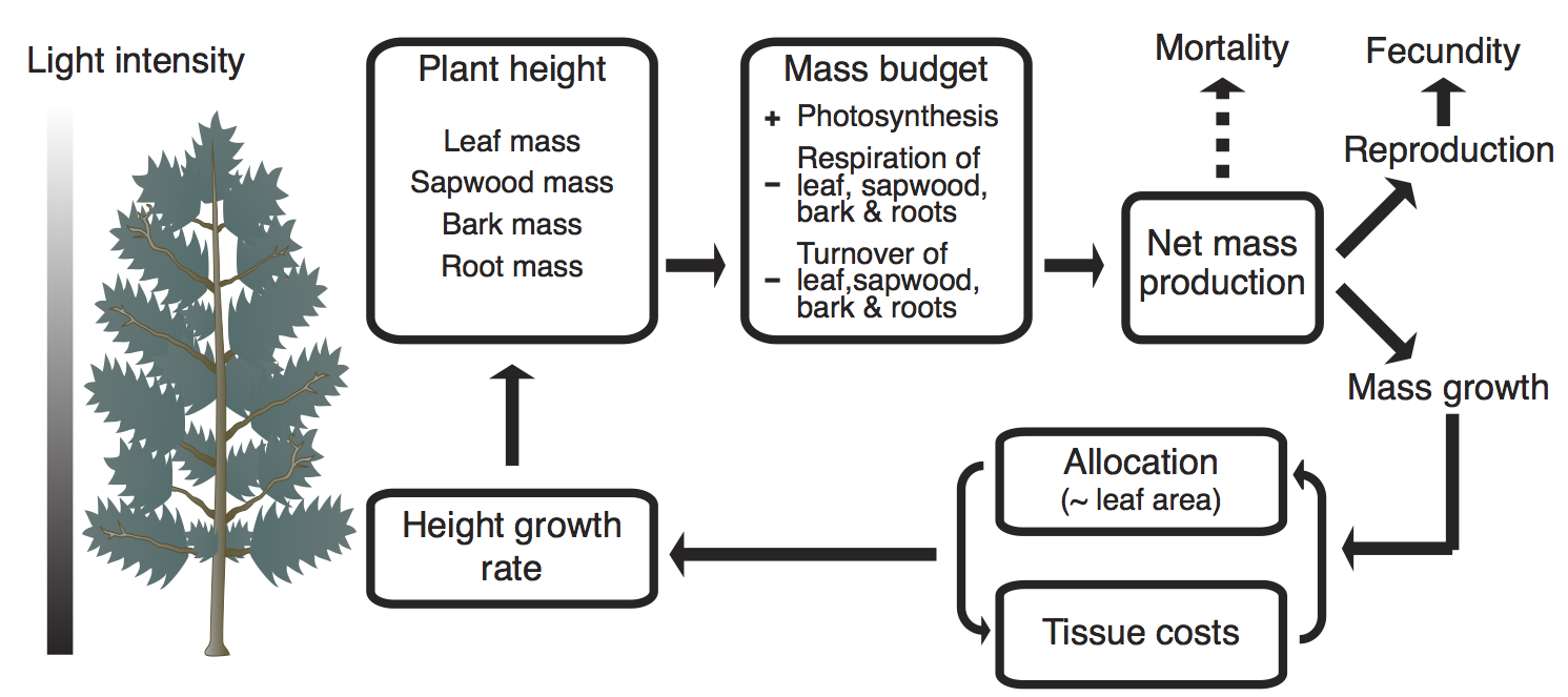
From these inputs, the model calculates how quickly the plant grows, how many seeds it produces, and how likely it is to die. All three rates share the same starting point: a carbon budget. Leaves capture carbon through photosynthesis, while respiration and tissue turnover use some of that income. The carbon that remains is net biomass production. FF16 then divides this production between growth and reproduction, and uses poor production as a signal of increased mortality risk.
This shared carbon budget is important. Growth, reproduction, and mortality are not three unrelated assumptions; they are different consequences of the same plant physiology. Size and traits affect both sides of the budget. For example, a larger plant can carry more leaves and capture more light, but it also has more living tissue to maintain.
The rest of this page develops that idea mathematically. The model was developed elsewhere, particularly in Falster, Brännström, Dieckmann, & Westoby (2011). The equations are collected here so that users can see the complete FF16 system implemented in plant, not as a claim that the model originated in this documentation.
Introduction
A physiological model in plant connects an individual plant to the wider population model. It takes the individual’s size, light environment, and physiological parameters as inputs, and returns three vital rates: growth, mortality, and fecundity.
In FF16, net biomass production links these inputs to all three outputs (Figure 1). Physiological parameters determine how the plant earns carbon, what it costs to maintain its tissues, and how it divides the remaining production. Changing those parameters can therefore represent differences among species. The Tables section defines the variables and lists the default parameter values used by the implementation.
Growth
Leaf photosynthesis
We begin with photosynthesis by a small patch of leaf. Let \(x\) denote the plant’s traits, \(z\) a height within its crown, and \(E(z)\) the light available at that height. The gross photosynthetic rate per unit leaf area is \(p(x,E)\), which FF16 represents with a saturating light-response curve: \[
p(x, E(z)) = \alpha_{{\rm p1}} \frac{ E(z)}{E(z) + \alpha_{{\rm p2}}},
\tag{1}\] Here, \(\alpha_{{\rm p1}}\) is the maximum annual photosynthetic rate, and \(\alpha_{{\rm p2}}\) is the light level at which the leaf reaches half that maximum. Both parameters are derived from a more detailed leaf-level model.
Leaves at different heights receive different amounts of light. To obtain a whole-plant average, the model weights the photosynthetic rate at each height by the fraction of the plant’s leaf area found there: \[
\bar{p}(x, H, E_{a}) = \int_0^H p(x, E_a(z)) \, q(z, H) \, {\rm d}z,
\tag{2}\] where \(H\) is plant height and \(q(z,H)\) describes the vertical distribution of leaf area (Equation 14). The result, \(\bar p\), is the mean photosynthetic rate per unit leaf area across the whole crown.
Mass production
The next step is to turn photosynthesis into net biomass production. The accounting is much like a budget: total photosynthesis is the income, while maintenance respiration and tissue turnover are expenses (Mäkelä, 1997; Thornley & Cannell, 2000; Falster et al., 2011). Their balance gives \({\rm d}B/{\rm d}t\): \[
\underbrace{\strut \frac{{\rm d}B}{{\rm d}t}}_\textrm{net biomass production}
= \underbrace{\strut \alpha_{\rm bio} }_\textrm{mass per C} \,
\underbrace{\strut \alpha_{\rm y} }_\textrm{yield}
\big( \underbrace{\strut A_{\rm l} \, \bar{p}}_\textrm{photosynthesis} -
\underbrace{\strut \, \sum_{i = {\rm l}, {\rm b}, {\rm s}, {\rm r}}{M_i \, r_i}}_\textrm{respiration}\big)
- \underbrace{\strut \sum_{i = {\rm l}, {\rm b}, {\rm s}, {\rm r}}{M_i \, k_i}}_\textrm{turnover}.
\tag{3}\] The tissue subscripts are \(l\) for leaves, \(b\) for bark, \(s\) for sapwood, and \(r\) for roots. For each tissue, \(M_i\) is its mass, \(r_i\) its maintenance respiration rate, and \(k_i\) its turnover rate. The other terms make two conversions:
- \(\alpha_{\rm y}\) is the fraction of assimilated carbon retained after growth respiration; and
- \(\alpha_{\rm bio}\) converts retained carbon into biomass.
Total photosynthesis equals the mean rate per unit leaf area, \(\bar p\), times total leaf area, \(A_{\rm l}\). Leaf area is related to leaf mass by \(A_{\rm l}=M_{\rm l}/\phi\), where \(\phi\) is leaf mass per area. The total living mass that the plant must support is \(M_{\rm a}=M_{\rm l}+M_{\rm b}+M_{\rm s}+M_{\rm r}\).
Height growth
The demographic model tracks individuals by height, so it needs to translate net biomass production into height growth. FF16 makes this conversion in three conceptual steps: production builds living tissue, living tissue supports leaf area, and leaf area is related to height. The chain rule combines these steps (Falster et al., 2011): \[
g(x, H, E_{a}) = \frac{{\rm d}H}{{\rm d}t} = \frac{{\rm d}H}{{\rm d}A_{\rm l}}
\times \frac{{\rm d}A_{\rm l} }{{\rm d}M_{\rm a}}
\times \frac{{\rm d}M_{\rm a}}{{\rm d}B}
\times \frac{{\rm d}B}{{\rm d}t}.
\tag{4}\]
Read from right to left, the four factors ask:
- How much net biomass does the plant produce?
- What fraction of that production becomes new living tissue rather than reproductive tissue?
- How much additional leaf area can that living tissue support?
- How much taller does the plant become for that increase in leaf area?
The final factor, \({\rm d}H/{\rm d}A_{\rm l}\), captures plant architecture. Some species deploy relatively more leaf area, whereas others gain relatively more height from the same increase in leaf area.
The term \({\rm d}A_{\rm l}/{\rm d}M_{\rm a}\) represents the marginal cost of deploying more leaf area. A plant must build not only the new leaves, but also the sapwood, bark, and roots needed to support them. The inverse of those combined construction costs is \[
\frac{{\rm d}A_{\rm l}}{{\rm d}M_{\rm a}}
= \bigg( \frac{{\rm d}M_{\rm l}}{{\rm d}A_{\rm l}} + \frac{{\rm d}M_{\rm s}}{{\rm d}A_{\rm l}} + \frac{{\rm d}M_{\rm b}}{{\rm d}A_{\rm l}} + \frac{{\rm d}M_{\rm r}}{{\rm d}A_{\rm l}}\bigg)^{-1}.
\tag{5}\]
The remaining conversion, \({\rm d}M_{\rm a}/{\rm d}B\), is the fraction of net biomass production allocated to growth rather than reproduction. FF16 assumes that young plants allocate nearly all production to growth, then shift more production towards reproduction as they approach their maturation height: \[
\frac{{\rm d}M_{\rm a}}{{\rm d}B}(H) = 1 -
\frac{\alpha_{{\rm f1}}} {1 + \exp\left(\alpha_{{\rm f2}} \left(1 - H / H_{\rm mat}\right)\right)},
\tag{6}\] Here, \(\alpha_{{\rm f1}}\) is the maximum fraction allocated to reproduction (between 0 and 1), \(\alpha_{{\rm f2}}\) controls how abruptly allocation changes, and \(H_{\rm mat}\) sets the height around which the transition occurs (Falster et al., 2011).
Diameter growth
Although height is the size variable used in the population model, FF16 can also calculate stem diameter. Total stem basal area, \(A_{\rm st}\), is the sum of sapwood, bark, and heartwood cross-sectional areas (\(A_{\rm s}\), \(A_{\rm b}\), and \(A_{\rm h}\)). Its rate of change is therefore \[
\frac{{\rm d}A_{\rm st}}{{\rm d}t} = \frac{{\rm d}A_{\rm b}}{{\rm d}t} + \frac{{\rm d}A_{\rm s}}{{\rm d}t} + \frac{{\rm d}A_{\rm h}}{{\rm d}t}.
\tag{7}\]
Basal-area growth uses the same production, allocation, and construction terms as height growth. It also includes the conversion of sapwood to heartwood: \[
\frac{{\rm d}A_{\rm st}}{{\rm d}t} = \left(\frac{{\rm d}A_{\rm s}}{{\rm d}A_{\rm l}} + \frac{{\rm d}A_{\rm b}}{{\rm d}A_{\rm l}}\right) \times
\frac{{\rm d}A_{\rm l}}{{\rm d}M_{\rm a}} \times \frac{{\rm d}M_{\rm a}}{{\rm d}B} \times \frac{{\rm d}B}{{\rm d}t} + \frac{{\rm d}A_{\rm h}}{{\rm d}t} .
\tag{8}\] Finally, the geometric relationship between stem area and diameter converts basal-area growth into diameter growth: \[
\frac{{\rm d}D}{{\rm d}t} = \left(\pi \, A_{\rm st}\right)^{-0.5} \, \frac{{\rm d}A_{\rm st}}{{\rm d}t}.
\tag{9}\]
Functional-balance model for allocation
The previous section used tissue masses and areas even though the population model tracks only plant height. FF16 connects these quantities through an allometric functional-balance model. Given a plant’s height, the model infers how much leaf, sapwood, bark, and fine-root tissue it needs to maintain a workable plant architecture.
This approach keeps the population model one-dimensional while still charging the plant for all the tissue needed to support new leaves. It also allows the growth rates of individual tissues to be derived from height growth (Table 2).
Leaf area
The first relationship links total leaf area to height. Following empirical allometry (Falster et al., 2011), FF16 uses a power law: \[
H = \alpha_{{\rm l1}} \, \left(A_{\rm l} \, {\rm m^{-2}}\right)^{\alpha_{{\rm l2}}}.
\tag{10}\] The factor \({\rm m^{-2}}\) makes the quantity inside the power dimensionless, so the relationship is normalised at a leaf area of 1 m\({^2}\).
Vertical distribution of leaf area
Total leaf area is not enough to calculate photosynthesis: the model also needs to know where those leaves sit within the crown. FF16 follows Yokozawa & Hara (1995) and describes crown shape with a single parameter, \(\eta\). Setting \(\eta=1\) gives a conical canopy, as seen in many conifers. A larger value, such as \(\eta=12\), produces a more top-heavy crown like those of many angiosperms.
Let \(A_{{\rm s},z}\) be sapwood area at height \(z\), and let \(A_{\rm s}\) be sapwood area at the base of the plant. Following Yokozawa & Hara (1995), their relationship is \[
\frac{A_{{\rm s},z}}{A_{\rm s}} = \left(1 - \left(\frac{z}{H}\right)^\eta\right)^2.
\tag{11}\]
The pipe model assumes that each unit of leaf area is supported by a fixed area, \(\theta\), of sapwood (Shinozaki, Yoda, Hozumi, & Kira, 1964). Basal sapwood area is therefore proportional to total leaf area: \[
A_{\rm s} = \theta \, A_{\rm l}.
\tag{12}\] FF16 applies this relationship both within an individual and across plants of different sizes. As a result, the fraction of a plant’s leaves above height \(z\), denoted \(Q(z,H)\), is
\[
Q(z, H) = \left(1-\left(\frac{z}{H}\right)^\eta\right)^2.
\tag{13}\]
Differentiating this cumulative relationship gives \(q(z,H)\), the density that describes how leaf area is distributed with height: \[
q(z, H) = 2\frac{\eta}{H}\left(1-\left(\frac{z}{H}\right)^{\eta}\right) \left(\frac{z}{H}\right)^{\eta-1}.
\tag{14}\]
Sapwood mass
Sapwood mass depends on its cross-sectional area throughout the full height of the stem. Integrating \(A_{{\rm s},z}\) over height and multiplying by wood density, \(\rho\), gives \[
M_{\rm s} = \rho \int_0^H A_{{\rm s},z} \, {\rm d}z = \rho A_{\rm s} H \eta_{\rm c} ,
\tag{15}\] where \(\eta_{\rm c} = 1 - \frac{2}{1 + \eta} + \frac{1}{1 + 2\eta}\) is a factor determined by crown shape (Yokozawa & Hara, 1995). Substituting the pipe-model relationship from Equation 12 expresses sapwood mass directly in terms of leaf area and plant height: \[
M_{\rm s} = \rho \, \eta_{\rm c} \, \theta \, A_{\rm l} \, H.
\tag{16}\]
Bark mass
FF16 treats bark and phloem with a relationship analogous to the pipe model. Their mass is a fixed fraction, \(\alpha_{{\rm b1}}\), of sapwood mass: \[
M_{\rm b} = \alpha_{{\rm b1}} M_{\rm s}.
\tag{17}\]
Root mass
Root mass is also proportional to leaf area: \[
M_{\rm r} = \alpha_{{\rm r1}} \, A_{\rm l}.
\tag{18}\] FF16 does not explicitly model nitrogen or water uptake. This relationship nevertheless ensures that building and maintaining roots contributes to the plant’s carbon budget.
Seed production
Once the plant begins reproducing, the fraction of production not allocated to growth is available for seeds. Dividing that reproductive production by the total cost per seed gives the seed-production rate, \(f(x,H,E_a)\): \[
f(x, H, E_{a}) = \frac{(1 - \frac{{\rm d}M_{\rm a}}{{\rm d}B}) \times \frac{{\rm d}B}{{\rm d}t}}{
\omega + \alpha_{{\rm f3}}},
\tag{19}\] Here, \(\omega\) is seed mass and \(\alpha_{{\rm f3}}\) is the additional cost of flowers, fruits, and dispersal structures associated with each seed. From Equation 6, \({\rm d}M_{\rm a}/{\rm d}B\) is the fraction allocated to growth, so \(1-{\rm d}M_{\rm a}/{\rm d}B\) is the fraction allocated to reproduction.
Mortality
FF16 represents mortality as a continuous hazard: the instantaneous risk of death at a particular size and in a particular environment. The total hazard has two parts (Moorcroft, Hurtt, & Pacala, 2001; Falster et al., 2011): \[
d(x, H, E_{a}) = d_{{\rm I}}(x, H) + d_{{\rm G}}(x, H, E_{a}).
\tag{20}\] The growth-independent component, \(d_{\rm I}\), is constant with respect to current plant performance, although it may vary among trait combinations. The growth-dependent component, \(d_{\rm G}\), falls exponentially as net biomass production per unit leaf area increases: \[
d_{{\rm G}}(x, H, E_{a}) = \alpha_{{\rm dG1}} \exp(-\alpha_{{\rm dG2}} X),
\tag{21}\] where \(X=({\rm d}B/{\rm d}t)/A_{\rm l}\). Plants with little production relative to their leaf area therefore face a higher mortality hazard. The parameters \(\alpha_{{\rm dG1}}\) and \(\alpha_{{\rm dG2}}\) allow the level and sensitivity of this response to differ among species.
Germination and establishment require a separate survival function, \(S_{\rm G}(x^\prime,H_0,E_{{\rm a}0})\), evaluated for a new plant of initial height \(H_0\) in its initial environment \(E_{{\rm a}0}\). For the demographic model to remain well behaved, the ratio \(S_{\rm G}(x^\prime,H_0,E_{{\rm a}0})/g(x,H_0,E_{{\rm a}0})\) must approach zero as initial growth approaches zero. Following Falster et al. (2011), FF16 uses \[
S_{\rm G} (x^\prime, H_0, E_{{\rm a}0}) = \frac1{1 + X^2},
\tag{22}\] where \(X = \alpha_{{\rm d0}} \frac{A_{\rm l}}{{\rm d}B / {\rm d}t}\) and \(\alpha_{{\rm d0}}\) is a constant. Because \(X\) is large when production per unit leaf area is small, establishment survival falls towards zero for plants with very poor initial production. This is consistent with the growth-dependent mortality rule in Equation 21: both penalise poor carbon balance.
Hyper-parameterisation of physiological model via traits
FF16 has default values for every physiological parameter (Table 3), but species can differ substantially in quantities such as leaf mass per area (\(\phi\)), wood density (\(\rho\)), leaf nitrogen per area (\(\nu\)), and seed mass (\(\omega\)). These measurable quantities can therefore be used as functional traits that distinguish strategies.
A trait often affects more than one model parameter. For example, changing leaf mass per area alters both the cost of constructing leaf area and the rate at which leaves turn over. Treating those effects independently could create a plant strategy that violates an assumed biological trade-off.
To keep linked parameters consistent, plant hyper-parameterises FF16: trait values are passed through a set of relationships that update several physiological parameters together. Those relationships are described below. Their implementation is in the make_FF16_hyperpar() function.
Leaf mass per unit area
Leaf mass per unit area, \(\phi\), measures how much dry mass is needed to build a unit of leaf area. A larger \(\phi\) therefore increases the construction cost captured by \({\rm d}A_{\rm l}/{\rm d}M_{\rm a}\). It is also linked to leaf turnover through the widely observed relationship reported by Wright et al. (2004): \[
k_{\rm l} = \beta_{{\rm kl1}} \, \left(\frac{\phi}{\phi_0}\right)^{-\beta_{{\rm kl2}}}.
\tag{23}\]
Here, \(\phi_0\) is the global mean of \(\phi\). Normalising the relationship at \(\phi_0\) allows \(\beta_{{\rm kl1}}\) and \(\beta_{{\rm kl2}}\) to change its level and slope without shifting it away from the observed mean.
Leaf respiration is specified per unit leaf mass, but is constrained to remain constant per unit leaf area for a given leaf nitrogen content. It therefore varies with both \(\phi\) and nitrogen per unit leaf area, \(\nu\), following Wright et al. (2004): \[
r_{\rm l} = \frac{\beta_{{\rm lf4}}\, \nu}{\phi}.
\tag{24}\]
Wood density
Wood density, \(\rho\), affects how much biomass is needed to build a given volume of stem. It therefore changes the construction-cost term \({\rm d}A_{\rm l}/{\rm d}M_{\rm a}\). FF16 can also link wood density to the growth-independent mortality rate, \[
d_{\rm I} = \beta_{{\rm dI1}} \, \left(\frac{\rho}{\rho_0}\right) ^ {-\beta_{{\rm dI2}}},
\tag{25}\]
and to the sapwood turnover rate, \[
k_{\rm s} = \beta_{{\rm ks1}} \, \left(\frac{\rho}{\rho_0}\right)^ {-\beta_{{\rm ks2}}},
\tag{26}\]
where \(\rho_0\) is the global mean wood density. As with \(\phi\), normalising at this mean keeps the relationships anchored while their other parameters vary. By default, \(\beta_{{\rm dI2}}\) and \(\beta_{{\rm ks2}}\) are zero, so wood density does not affect these two rates unless the corresponding exponents are changed.
FF16 assumes that sapwood respiration is constant per unit volume. A unit of mass occupies less volume when wood is denser, so respiration per unit mass is \[
r_{\rm s} = \frac{\beta_{{\rm rs1}}}{\rho},
\tag{27}\]
where \(\beta_{{\rm rs1}}\) is the default respiration rate per unit sapwood volume. Bark respiration per unit mass follows the same logic: \[
r_{\rm b} = \frac{\beta_{{\rm rb1}}}{\rho},
\tag{28}\]
with \(\beta_{{\rm rb1}} = 2 \beta_{{\rm rs1}}\).
Seed mass
Seed mass, \(\omega\), directly affects fecundity through Equation 19 and also determines a seedling’s initial height. FF16 assumes that the accessory cost of producing flowers, fruits, and dispersal structures scales with seed mass: \[
\alpha_{{\rm f3}} = \beta_{{\rm f1}} \omega,
\tag{29}\] as observed empirically by Henery & Westoby (2001).
Nitrogen per unit leaf area
Leaf nitrogen per unit area, \(\nu\), affects both photosynthesis and respiration. The respiration relationship was introduced above. For photosynthesis, FF16 first calculates the instantaneous response of a leaf to light and then averages that response over an annual solar trajectory. The light-response curve is \[
p(\nu, E) = \frac1{365 \textrm{d}}\int_0^{365 \textrm{d}}\frac{Y(t) + A_{\rm max} - \sqrt{(Y(t) + A_{\rm max})^2 - 4 \beta_{{\rm lf2}} Y(t) A_{\rm max} }}{2 \beta_{{\rm lf2}}} {\rm d}t,
\tag{30}\] The terms in this expression are:
- \(A_{\rm max}\) is the maximum photosynthetic capacity of the leaf,
- \(\beta_{{\rm lf2}}\) is the curvature of the light response curve,
- \(Y(t) = \beta_{{\rm lf3}} I(t)\) is the initial yield of the light response curve, with \(\beta_{{\rm lf3}}\) being the quantum yield parameter,
- \(I(t) = k_{\rm I} \, I_0(t)\, E\) is the intensity of light on the leaf surface, and
- \(I_0(t)\) is light incident on a surface perpendicular to the sun’s rays directly above the canopy at time \(t\).
The time-varying profile \(I_0(t)\) comes from a solar model adapted from Ter Steege (1997).
Maximum photosynthetic capacity increases with leaf nitrogen per unit area according to \[
A_{\rm max} = \beta_{{\rm lf1}} \, \left(\frac{\nu}{\nu_0}\right)^{\beta_{{\rm lf5}}},
\tag{31}\] where \(\beta_{{\rm lf1}}\) and \(\beta_{{\rm lf5}}\) are constants, and \(\nu_0\) is the global mean leaf nitrogen per unit area used to normalise the relationship.
Finally, the model evaluates \(p(\nu,E)\) across a range of light levels and fits the simpler curve in Equation 1. This fitting step turns \(\alpha_{{\rm p1}}\) and \(\alpha_{{\rm p2}}\) into functions of leaf nitrogen. The rest of FF16 can then use the compact photosynthesis equation while retaining the effect of \(\nu\) derived from the detailed annual calculation.
Tables
The following tables collect the notation, allometric relationships, and parameter values used above. They are generated directly from the installed plant package so that the displayed defaults match the implementation.
References
Falster, D. S., Brännström, Å., Dieckmann, U., & Westoby, M. (2011). Influence of four major plant traits on average height, leaf-area cover, net primary productivity, and biomass density in single-species forests: A theoretical investigation.
Journal of Ecology,
99(1), 148–164. doi:
10.1111/j.1365-2745.2010.01735.x
Falster, D. S., Brännström, Åke, Westoby, M., & Dieckmann, U. (2015). Multi-trait eco-evolutionary dynamics explain niche diversity and evolved neutrality in forests.
bioRxiv, 014605. doi:
10.1101/014605
Henery, M., & Westoby, M. (2001). Seed mass and seed nutrient content as predictors of seed output variation between species.
Oikos,
92, 479–490. doi:
10.1034/j.1600-0706.2001.920309.x
Mäkelä, A. (1997). A carbon balance model of growth and self-pruning in trees based on structural relationships. Forest Science, 43, 7–24.
Moorcroft, P. R., Hurtt, G. C., & Pacala, S. W. (2001). A method for scaling vegetation dynamics: The
Ecosystem Demography model
(ED).
Ecological Monographs,
71(4), 557–586. doi:
10.1890/0012-9615(2001)071[0557:AMFSVD]2.0.CO;2
Shinozaki, K., Yoda, K., Hozumi, K., & Kira, T. (1964). A quantitative analysis of plant form - the pipe model theory. I. Basic analyses. Japanese Journal of Ecology, 14, 97–105.
Ter Steege, H. (1997).
Winphot 5: A programme to analyze vegetation indices, light and light quality from hemispherical photographs. Georgetown, Guyana: Tropenbos Guyana Programme. Retrieved from
http://www.researchgate.net/publication/230608417
Thornley, J. H. M., & Cannell, M. G. R. (2000). Modelling the components of plant respiration: Representation and realism.
Annals of Botany,
85(1), 55–67. doi:
10.1006/anbo.1999.0997
Wright, I. J., Reich, P. B., Westoby, M., Ackerly, D. D., Baruch, Z., Bongers, F., … Villar, R. (2004). The world-wide leaf economics spectrum.
Nature,
428, 821–827. doi:
10.1038/nature02403
Yokozawa, M., & Hara, T. (1995). Foliage profile, size structure and stem diameter plant height relationship in crowded plant-populations. Annals of Botany, 76(3), 271–285.