Once you’ve written the model down as a set of ordinary differential equations, the job of the solver is simple to describe even if the mechanics are intricate: start from the current state and march forward in time, one small step at a time, building up the future from the present. The question that makes this hard is how big each step should be. Take steps that are too large and the solution drifts away from the truth, accumulating error you can’t see until it’s too late. Take steps that are too small and you waste enormous amounts of computation grinding through periods where nothing much is changing. The solver used here resolves this by adapting as it goes. At every step it takes a trial step forward, then checks how much that step disagrees with a slightly more careful version of the same step. That disagreement is a proxy for the error being made. When the disagreement is small, the solver grows more confident and takes a longer stride next time. When it’s large, the solver backs off and takes a shorter, more cautious step. The result is a trajectory through time that spends its effort where growth and mortality are changing quickly, and coasts through the quiet periods, all while keeping the error in each step below a chosen tolerance. The rest of this page makes this precise.
plant casts the entire patch as a system of ordinary differential equations (ODEs) and steps it through time with classic ODE methods. (For details on the equations themselves see the size-structured PDE page.) This page first describes the Runge–Kutta solver and the Control() parameters that govern it, then works through the trade-off between the default adaptive stepper and a fixed-step forward-Euler mode using a work–precision diagram.
The Runge–Kutta 45 ODE stepper
The plant model uses an explicit Runge-Kutta ODE stepper to integrate the ordinary differential equations that describe the system. Specifically, we use the Runge-Kutta Cash-Karp 4-5 (RK45) algorithm, with adaptive time step.
In brief, this means that the solver takes a step through time, and then evaluates the error in the step. Error is estimated by comparing two possible steps: one using 4 sub-intervals, and one using 5 sub-intervals. By comparing the step made with more sub-intervals, the algorithm can estimate the non-linearity in the system and error in the step. If the error is too high, the solver will attempt to take a smaller step. If the error is well below a target value, the solver will attempt to take a larger step. Importantly, the 5 step reuses information from the 4 step and thereby only requires a single extra call on rates of change, so the RK45 algorithm is much more efficient than alternatives like the RK48. The math of RK45 stepping has long been established, and the method is available in most solvers for ODE systems. You can read more about Runge-Kutta methods and adaptive time steps on Wikipedia.
The RK45 is an explicit method, as opposed to an implicit method. As wikipedia explains“Explicit methods calculate the state of a system at a later time from the state of the system at the current time, while implicit methods find a solution by solving an equation involving both the current state of the system and the later one”. The advantage of explicit methods are that they are simple to implement and fast, particularly when allowing adaptive time steps. The disadvantage is that they are less stable than implicit methods when they encounter stiff systems. As described in wikipedia
“Implicit methods require an extra computation, and they can be much harder to implement. Implicit methods are used because many problems arising in practice are stiff, for which the use of an explicit method requires impractically small time steps \(\Delta t\) to keep the error in the result bounded”.
“Explicit Runge Kutta methods are generally unsuitable for the solution of stiff equations because their region of absolute stability is small; in particular, it is bounded. This issue is especially important in the solution of partial differential equations….. The advantage of implicit Runge–Kutta methods over explicit ones is their greater stability, especially when applied to stiff equations.”
In practice, we’ve found the RK45 to be extremely stable and fast for solving the size-density distribution. However, there are circumstances where the system becomes stiff and the solver struggles. E.g.
When implementing soil water into plant via the Richards Equation, Isaac Towers found the system became stiff.
When implementing the FF16 model in another solver, Joshi et al 2023 https://doi.org/10.1101/2023.08.04.551683 reported that the system became stiff when enabling a continuous feedback of seeds into germination.
Any extensions should therefore be wary of stiff behaviours.
Setup of templated ODE solver in C++
The characteristic method used to solve density requires regular introduction of new nodes, which entails a resizing of the ODE system as the system progresses. To make this play nicely with the ODE stepping, Rich FitzJohn designed a custom ODE solver class based on the RK45 method. The code is built into the model, with some details ported from the GNU Scientific Library(Galassi, 2009).
The main interface is the class odelia::ode::Solver. The solver has been extracted from plant into a standalone odelia library, so it no longer lives under inst/include/plant/; plant pulls it in via #include <odelia/ode_solver.hpp> (see scm.h). The class is established using a template System class, meaning you can effectively cast any variety of classes as an ODE Solver. (In a similar way, you can create a vector of any variety of data types.)
The main solver for our system is the class SCM, (in the file scm.h). This creates an ode solver based on patch type. Simultaneously, the class SCM owns an actual instance of the patch, which contains species and environment.
patch_type patch;# Instance of patchodelia::ode::Solver<patch_type> solver;# ODE solver (owns the system)
All we need to do to advance the system is make calls like the following. These advance the system, using the patch to estimate rates of change. Moreover, we can take steps of a specified fixed size, or an adaptive step where the solver determines the spacing. Note that the solver now owns the system, so these calls no longer take the patch as an argument — they operate on the system the solver already holds:
A third method, solver.advance_euler(...), backs the fixed-step forward-Euler mode (fixed_time_step, discussed below).
In the background, the solver then passes information (rates of change, states) between the actual patch (which contains all the biological information informing rates of change) and ode solver (which uses the RK45 math to calculate future states from rates of change).
Additionally, we have the following function, which resizes the ODE system after a node has been introduced.
solver.set_state_from_system()
For the above to work, the patch class (see patch.h) must have some essential functions used by the ODE system.
// * ODE interface// Caluclate size of ode system (number of equations).size_t ode_size()const;// How many auxiallary variables are we tracking. These are being collected but// are not part of core ode systemsize_t aux_size()const;double ode_time()const;// Retrieve ode state from patch and save into the ode solverode::iterator ode_state(ode::iterator it)const;// Retrieve ode rates from patch and save into the ode solverode::iterator ode_rates(ode::iterator it)const;// Retrieve auxillary variables and save into the ode solverode::iterator ode_aux(ode::iterator it)const;// Set state of patch, based on estimate of future state estimated by the solverode::const_iterator set_ode_state(ode::const_iterator it,double time);
Note the use of iterators. These enable state from a complicated data structure like a patch, to be converted into a vector, as needed by ode solver. And vice versa.
Solving individuals and other systems
As templated C++, we can use the odelia::ode::Solver class to step any “system” that has the requisite functions. In addition to patches, we also use the ode solver to run individual plants, given an environment. This is achieved by introducing a wrapper class plant::tools::IndividualRunner (in individual_runner.h), which handles the ownership semantics around the solver and the object it steps.
Like the patch system, IndividualRunner is templated — on a strategy T and an environment E — so we can set up a variety of systems.
IndividualRunner provides exactly the ode_size()/ode_state()/ode_rates()/ set_ode_state() interface the solver expects, so it can be handed to an odelia::ode::Solver to step an individual plant to a given size. This is available via the R functions grow_individual_..., which in turn use IndividualRunner.
The test suite also shows how to drive the solver directly on the classic Lorenz system (see tests/testthat/test-ode-euler.R).
Controls on ODE stepping
The RK45 ode solver is controlled by a set of parameters that determine how the solver steps through time.
As a simple example, we can step a system using the default values for ODE stepping:
library(plant)# configure a patch containing a single speciesp0 <-scm_base_parameters("FF16")p0$max_patch_lifetime <-5p <-add_strategies(p0, trait_matrix(0.0825, "lma"))# Controls on numerical methodsctrl <-Control()# runout <-run_scm(p, ctrl = ctrl)# number of stepslength(out$ode_times)
[1] 97
The precise times used by the solver are stored in out$ode_times, so the length of this object indicates the number of times used.
The number and timing of steps taken by the solver will vary with the controls on the ode solver. Looking at the ctrl object, we can extract the items beginning with ode_, which control the ODE solver:
ode_step_size_initial: The initial step size used by the solver in the first step.
ode_step_size_min, ode_step_size_max: The minimum step size permitted. Any attempt by the solver to use a smaller value will be curtailed at this value.
ode_tol_abs, ode_tol_rel: When taking a step, the absolute and relative error for any single equation that is allowed. If the error is too high, the solver will attempt to take a smaller step. If the error is well below this value, the solver attempts to expand the step size in the next step.
ode_a_y, ode_a_dydt: Weightings on y and dy/dt, in calculation of allowable relative error (see OdeControl::errlevel).
Varying these will potentially change the number of steps taken by the solver.
However, note that unlike a regular ode solver, the number of steps taken is also influenced by the timing of node introduction. The ode stepper will only expand the time step up until the next node introduction event, for any species. So the node scheduling sets an upper limit on the size of time steps. In the default setup, the node schedule primarily determines the timesteps in the first months of the simulation. After that, the ode stepper takes a bigger control.
Limiting the Minimum and Maximum step size
Let’s alter the maximum step size and compare to what we had above.
The options above still drive the full adaptive RK45 machinery at each step. For operational-realism comparisons with daily-step DGVMs, plant can instead use plain forward (explicit) Euler on a uniform grid — one derivative evaluation per step, no error estimate — by setting fixed_time_step (units: years) on the Control:
This is not the way to get an accurate or cheap solution: forward Euler is first-order, and matching the adaptive solver’s accuracy needs far more evaluations. The next part works this trade-off through with a work–precision diagram. Note that fixed_time_step is incompatible with the mutant-fitness replay path (save_RK45_cache / use_ode_times) and errors clearly if combined.
Future changes
Would it help to have option to pass in ode_times, use if supplied?
But, current system in NodeSchedule interweaves ode_times and node_schedule_times. It’s complex code, poorly documented, low value to mess with. Suggests leaving as is
could have option to pass in ode_times, add to pars inside function, use if supplied?
if supplied, do we always want to use ode_times?
what’s the advantage of using previous ode_times?
suggest always using them if present?
Adaptive vs fixed-step
By default, plant integrates the patch with the adaptive, error-controlled Cash–Karp Runge–Kutta (RK45) stepper described above. The solver chooses each step size to keep the local error within a tolerance: tiny steps early on, when newly introduced cohorts are diverging rapidly, and much coarser steps later, once the stand settles.
Many widely used dynamic global vegetation models (DGVMs) instead march the state forward on a fixed grid — most commonly a daily time step — using plain forward (explicit) Euler. plant can be run this way too, via the fixed_time_step control (option 3 above). This part shows how to enable it and uses a work–precision diagram to make the central trade-off concrete: at matched accuracy, adaptive stepping does far less work.
library(plant)library(dplyr)library(ggplot2)
Enabling fixed-step forward Euler
The integration mode is selected by a single control field, fixed_time_step (units: years):
fixed_time_step = 0 (the default) → adaptive RK45.
fixed_time_step > 0 → forward Euler on a uniform grid of that spacing.
A daily step is therefore fixed_time_step = 1 / 365.
Forward Euler does one derivative evaluation per step (y <- y + h * dy/dt), whereas each RK45 step evaluates the derivatives six times. The two runs report slightly different fitness, and use a very different number of steps:
Caution — don’t read this as “Euler is faster”. A single daily step is cheaper than a single adaptive step (1 derivative evaluation versus 6), so a naive timing race makes Euler look quick. But that comparison holds the step count fixed, not the accuracy. Daily Euler here is visibly less accurate than the adaptive run. The honest question is: how much work does each method need to reach the same accuracy? That is what the work–precision diagram below answers — and there adaptive wins comfortably.
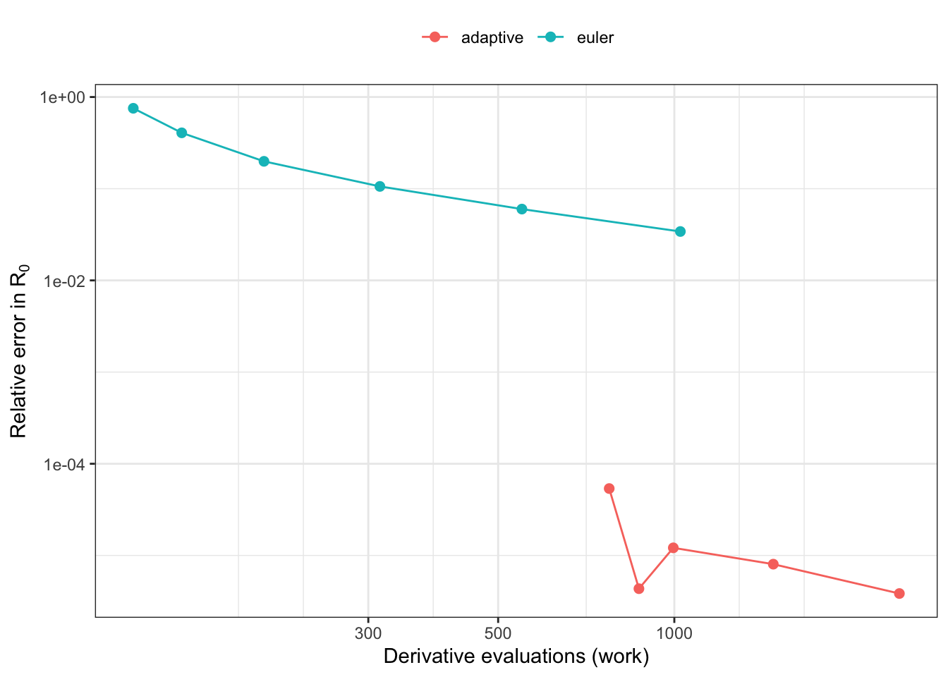
A work–precision diagram
We sweep the adaptive solver over a range of error tolerances, and forward Euler over a range of step sizes, and for each run record:
work: total derivative evaluations — 6 × n_steps for RK45, 1 × n_steps for Euler (this is the dominant cost of the inner loop);
error: relative error in the net reproduction ratio \(R_0\) against a tight-tolerance adaptive reference.
Figure 1: Work-precision diagram. Lower and to the left is better (less work, smaller error). The adaptive RK45 frontier sits well below the fixed-step Euler frontier: for any target accuracy it reaches it with fewer derivative evaluations.
Why adaptive stepping dominates
The two curves tell a consistent story:
Forward Euler is first-order. Halving the step size roughly halves the error, so the Euler curve descends slowly — buying an extra digit of accuracy costs roughly a tenfold increase in work.
Adaptive RK45 is high-order and adaptive. It spends small steps only where the dynamics demand them (the first weeks, while cohorts diverge) and coarsens dramatically once the stand stabilises. It reaches an error floor — set by the node-introduction schedule rather than the ODE tolerance — at a fraction of the evaluations Euler would need to match it.
To get daily-Euler accuracy down to the adaptive frontier you would need a sub-daily step everywhere, including the long, smooth tail of the simulation where the adaptive solver is happily taking steps of years. That is wasted work, and it is exactly the inefficiency adaptive stepping removes.
The practical conclusion: fixed-step Euler is valuable for operational-realism comparisons — running plant on the same footing as a daily-step DGVM — but it is not the way to get an accurate or cheap solution. For that, keep the default adaptive solver.
A run that completes is not a run that converged
Fixed-step integration removes the solver’s safety net: forward Euler will march across anything, including a discontinuous right-hand side that the adaptive solver rightly refuses. When that happens the integrator still returns numbers — but they are an artefact of where the step grid happens to fall, not an approximation to a solution that gets better as you refine.
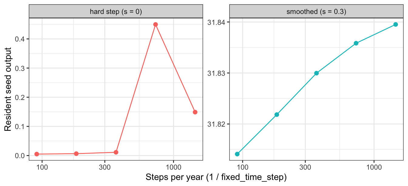
plant’s experimental PPA hard-step shading variant (ppa_layer_smoothing = 0, the literal field discretisation) is exactly such a case: its light profile is discontinuous in height, so the adaptive solver fails with “Cannot achieve the desired accuracy”. Under a fixed step it runs. The test of whether that result means anything is convergence: does it settle as the step shrinks? We compare it with the smoothed variant (ppa_layer_smoothing = 0.3), which is a well-posed, continuous problem.
ggplot(convergence, aes(steps_per_year, seed, colour = variant)) +geom_line() +geom_point(size =2) +facet_wrap(~variant, scales ="free_y") +scale_x_log10() +labs(x ="Steps per year (1 / fixed_time_step)", y ="Resident seed output",colour =NULL) +theme_bw() +theme(legend.position ="none")
Figure 2: Resident seed output as the fixed step shrinks. The smoothed variant converges; the hard step does not — it wanders by an order of magnitude with no limit. Note the independent y-scales: the hard step’s values are ~1000x smaller, and erratic. A result that depends on the step size is a property of the grid, not of the model.
The smoothed variant marches monotonically toward a limit — refining the step buys accuracy, as it should. The hard step does not converge to anything: each step size gives a different answer, so no step size gives the answer. This is why such variants must not be read as fitness or as a solution — the fixed-step solver makes them executable, not correct.
Caveats and scope
Mutant fitness / resident replay is not supported under fixed_time_step. The mutant pathway replays a resident run by reusing the six cached RK sub-step environments per step; forward Euler has a single stage and no such cache. Combining fixed_time_step > 0 with save_RK45_cache (or with a pinned use_ode_times replay) raises a clear error rather than returning a wrong fitness.
Discontinuous/“hard-step” environment variants only run to completion under a fixed grid and do not converge as the step shrinks (see the section above) — any apparent result is a grid artefact, not a solution. Do not interpret such runs as fitness or as a converged answer.
References
Galassi, M. (Ed.). (2009). GNU scientific library: Reference manual (3. ed., for GSL version 1.12). s.l.: Network Theory.