Self-thinning

example

In a recently cleared stand, a new cohort of saplings will emerge and start to grow, increasing in size, and eventually reaching a crowded state whereby all incoming light is being intercepted by the plants. At this point there will be very strong competition for light between individuals, and some plants will become taller than others, thus out-competing them. Some of those smaller plants will have insufficient growth to survive, and will eventually die.

This process of growth-dependent mortality is known as “self-thinning”, and can be equally understood as a size-density relationship, essentially resulting from the growth, survival and reproductive processes of the evolving stand, with the “self-thinning line” (STL) being an emergent outcome. Self-thinning is a widely documented empirical phenomenon, observed in many forest types around the world.

The STL is thought to be constant across stands, though there is conflicting evidence on the generality of the “law” across species, environments and stand types. The typical STL can be captured in plant by using the output of a stand simulation to determine mean size and mean density, per unit area and parameterised by time, which are plotted on a double-log scale and show a typically linear trajectory.

library(plant)
library(dplyr)
library(ggplot2)

plant_log_console()

[2026-06-21 17:21:34.263] Activating logging to console

Grow a stand of plants with the default parameters of the plant “FF16” model:

p0 <- scm_base_parameters("FF16")

p0$strategy_default$recruitment_decay <- 5
#stops seeds continuing to come into the stand from early on to isolate first "group" of plants that emerges around the same time

p0$control$schedule_eps <- 0.005
# more refined scheduling

lma_trait <- trait_matrix(0.1457419, "lma")

p1 <- expand_parameters(p0, trait_matrix = lma_trait)

stand_results <- run_scm(p1, refine_schedule = TRUE)$parameters
# creates a schedule for time steps when running the model, with many "steps" early on and fewer as the stand ages and doesn't change as rapidly

out <- run_scm(stand_results, collect = TRUE)
# run the SCM model

run_scm(..., collect = TRUE) already returns the output in a tidy format (a list whose species element is a tibble with all state variables as separate columns), so we can use it directly to calculate totals and mean values for the properties of the stand.

tidy_stand <- out

stand_expand <- FF16_expand_state(tidy_stand)
# adds in more state variables from our stand output (leaf, bark, sapwood, stem properties to name a few)

patch_total <-
    stand_expand$species %>%
    integrate_over_size_distribution() %>%
    mutate(
      # create average sizes
      across(c(diameter_stem, area_stem, area_leaf, height, mass_above_ground), ~.x/density,
             .names = "{.col}_av"))
# this gives us a final table of all the metrics gathered from the stand, and creates variables of averages calculated for leaf area, stem size (including the mean stem diameter that we need), height & biomass

Plot the STL: mean stem diameter (m) against density, per square meter, with log-scaled axes

patch_total %>%
    ggplot(aes(diameter_stem_av, density)) +
             geom_line() +
             scale_x_log10() +
             scale_y_log10() +
             xlab("stem diameter (m)") +
             ylab("density " ~(m^2)) +
             ggtitle("Self-thinning plot") +
             theme_classic(base_size = 18)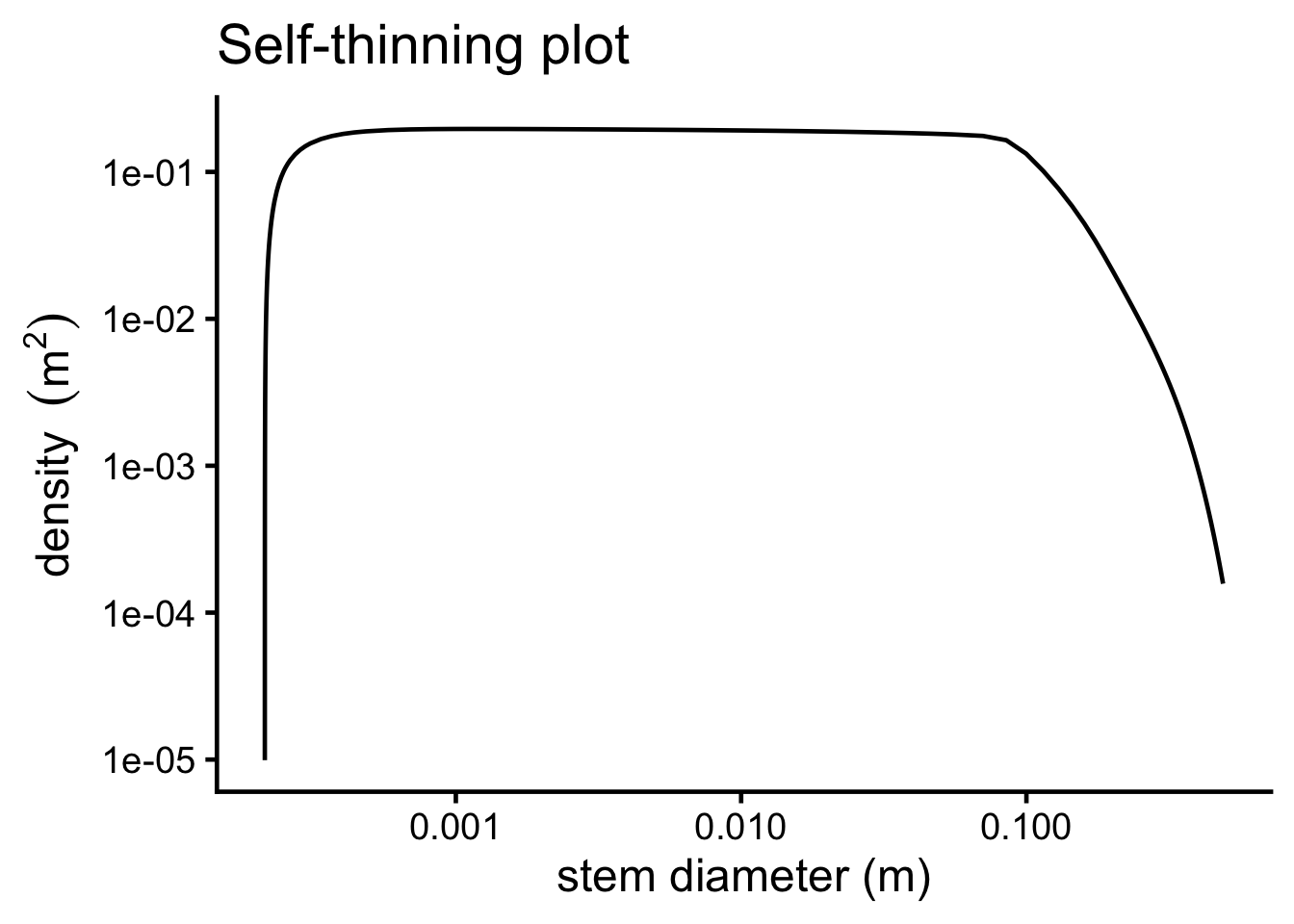

We can also plot other variables such as biomass and leaf area, to better understand the stand’s development

patch_total %>%
      ggplot(aes(time, area_leaf)) +
               geom_line() +
               xlab("time (yr)") +
               ylab("leaf area " ~(m^2)) +
               ggtitle("Leaf Area over time") +
               theme_classic(base_size = 18)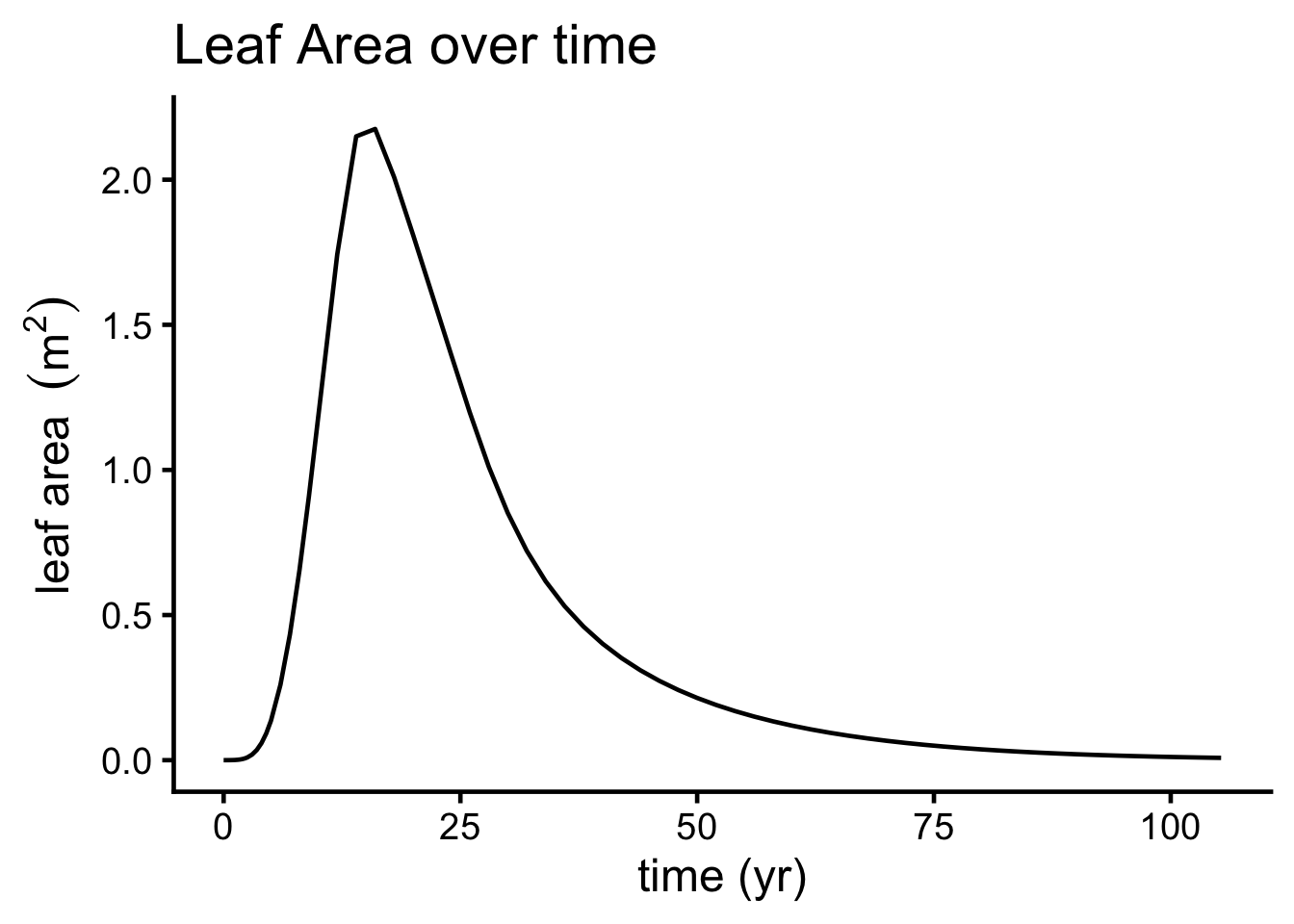

patch_total %>%
    ggplot(aes(time, mass_above_ground)) +
             geom_line() +
             xlab("time (yr)") +
             ylab("above-ground biomass (kg)") +
             ggtitle("Above-ground Biomass over time") +
             theme_classic(base_size = 18)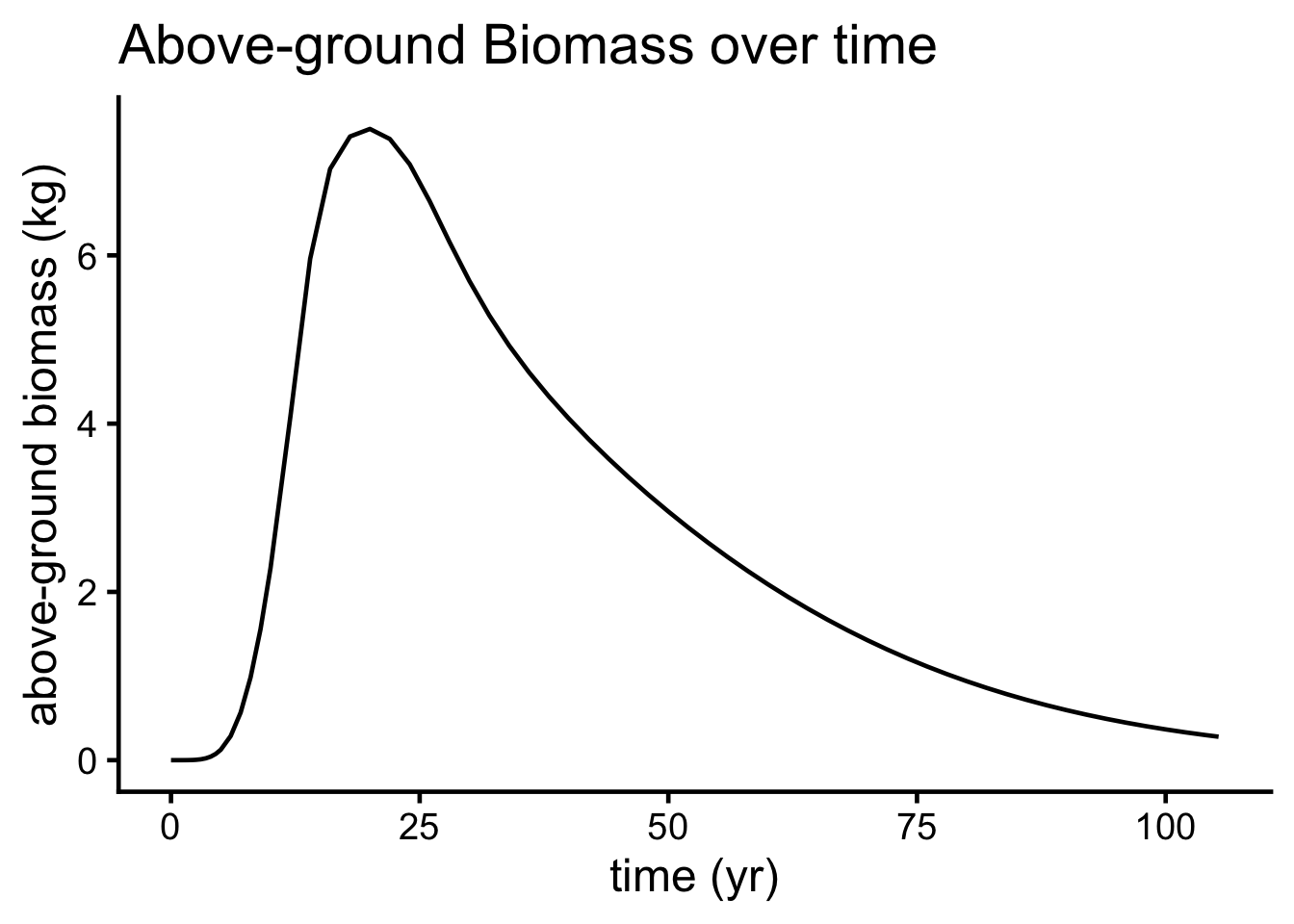

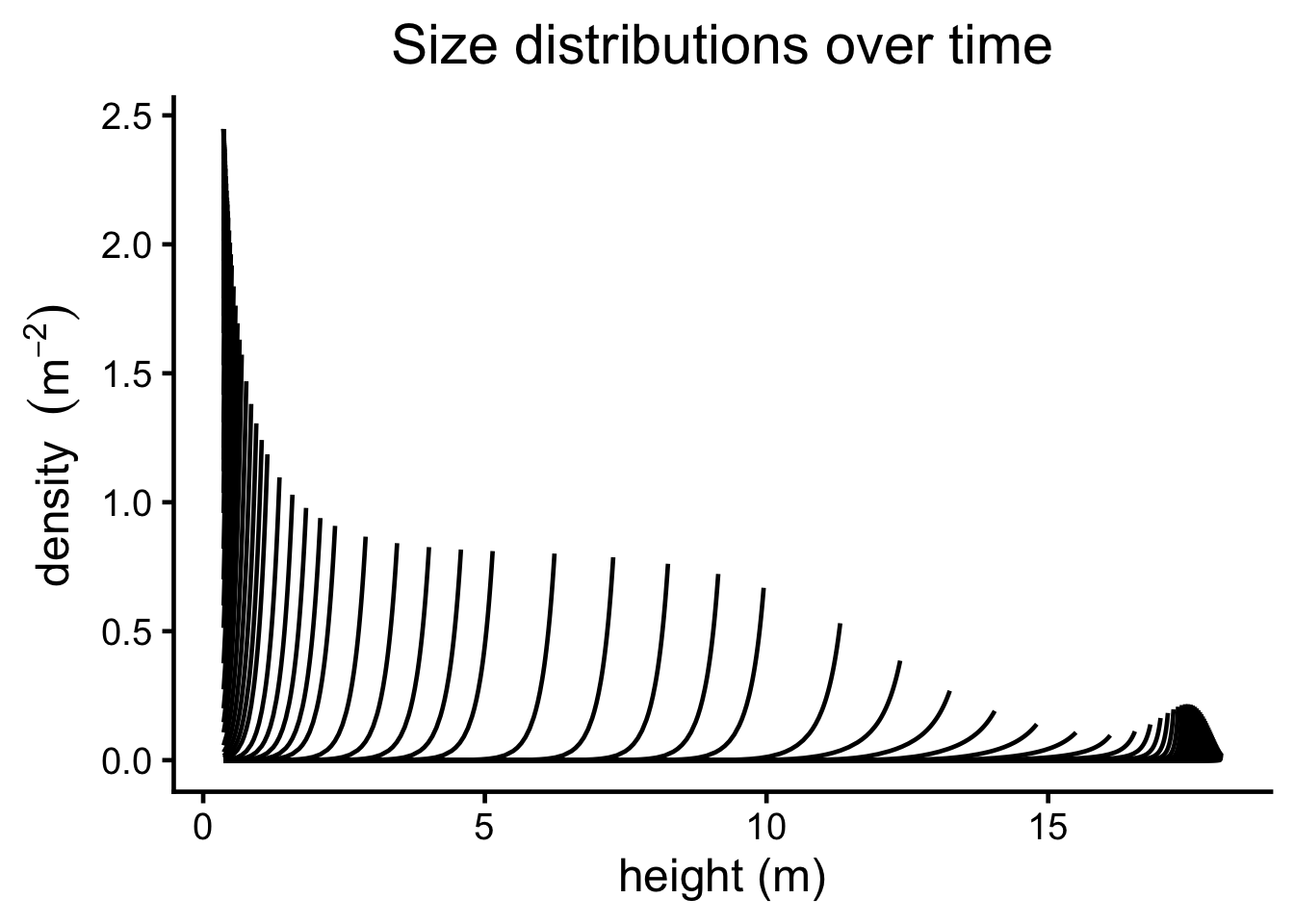
Finally, we can plot the height-density distribution evolving through time, as plant generates a size-distribution at each instance in time that the solver runs

Extracting and highlighting a few specific time points, we can see more clearly how the stand has developed. Initially there is a higher density of saplings that have emerged, with less height variation across the distribution. The population continually reduces in number as mortality is occurring, with greater size variation emerging as asymmetric competition for light is occurring, which benefits the taller plants the most. There is a narrower range of heights in the final distribution, which is late in the stand’s development, at ~ 98 years.

times <- tidy_stand$species$time[c(10500, 12000, 13000, 13500, 14000, 15000, 17000, 20000)]

# give explicit rows from time column to highlight

# find closest times to a given vector of times for labelling selected size distributions
find_closest <- function(x, at){
  out <- rep("", length(x))

  for(a in at){
    dist <- abs(x-a)
    i <- which(dist == min(dist))
    out[i] <- a
  }
  out
}

data_sub <- tidy_stand$species %>%
  mutate(my_label = find_closest(round(time, 2), at = c(0.5, 2, 5, 9, 14, 28, 56, 98))) %>%
  na.omit() %>%
  filter(time %in% times)

data_sub2 <- data_sub %>% group_by(time) %>% slice(1) %>% ungroup()

tidy_stand$species %>%
  ggplot(aes(height, density, group=time)) +
  geom_line() +
  geom_line(data = data_sub, col="blue") +
  geom_text(data = data_sub2, aes(label = my_label), nudge_y = 0.05, col="blue") +
  xlab("height (m)") +
  ylab("density " ~(m^-2)) +
  ggtitle("Size distributions over time") +
  theme_classic(base_size = 18) +
  theme(plot.title = element_text(hjust = 0.5))