library(plant)
library(dplyr)
library(tidyr)
library(ggplot2)
library(patchwork)Example analysis
example
This is the flagship end-to-end example: set up parameters, run a patch with the size-structured model, then summarise, integrate, and interpolate the results.
NoteRunning the
TF24 model needs a configured soil-water environment
The TF24 strategy couples plant growth to a multi-layer soil-water balance, so — unlike FF16 — it cannot run against a bare Environment("TF24"). The soil column must be given a number of layers and an initial moisture state, and the rainfall driver must keep the mean high enough that a layer never dries to zero (where the retention curve psi_from_soil_moist goes non-finite and the run aborts with set_physiology received non-finite psi_soil). We wrap that setup in make_tf24_env() below. Runtime is dominated by the hydraulic solver and scales with max_patch_lifetime, so this page pins it short (max_patch_lifetime = 25) to keep the build fast; raise it for production runs. The recipe follows the test-root vignette in the plant package.
installation
Activate logger
plant_log_console()We pin the patch lifetime short and define a helper that builds a TF24 environment with an initialised soil column (15 layers at moisture 0.2) and a seasonal rainfall driver with mean 1.0 — see the note above for why this is required.
max_patch_lifetime <- 25

make_tf24_env <- function(max_patch_lifetime, n_layers = 15, theta0 = 0.2) {
  env <- Environment("TF24")
  env$set_soil_number_of_depths(n_layers)
  env$set_soil_water_state(rep(theta0, n_layers))

  # seasonal rainfall; mean 1.0 keeps the column from drying to a non-finite psi
  x <- seq(0, max_patch_lifetime, length.out = 1000)
  y <- 0.25 * sin(2 * pi * x) + 1.0
  env$extrinsic_drivers_set_variable("rainfall", x = x, y = y)

  env
}
Very minimalist
p0 <- scm_base_parameters("TF24", "TF24_Env")
p0$max_patch_lifetime <- max_patch_lifetime

traits <- trait_matrix(c(0.07), c("lma"))

p1 <- add_strategies(p0, traits)

env <- make_tf24_env(max_patch_lifetime)

results <- run_scm(p1, env = env, refine_schedule = TRUE)$parameters
results <- run_scm(results, env = env, collect = TRUE)
This uses the default parameters in plant. But you may want alter some of the defaults. For that we recommend setting up some functions to set base_parameters.
base_parameters <- function() {
  p0 <- scm_base_parameters("TF24", "TF24_Env")
  p0$max_patch_lifetime <- max_patch_lifetime

  p0$strategy_default$pars$hmat <- 15
  p0$strategy_default$pars$rho <- 700
  p0$strategy_default$pars$a_l1 <- 2.17
  p0$strategy_default$pars$a_l2 <- 0.5

  p0
}
We can now create a second function called run_mypatch which takes a number of a arguments, including traits which we assign a trait matrix. The add_strategies function takes this trait matrix as an argument which allows us to simulate patches with multiple functional strategies, in addition to the base_parameters and any newly defined hyperparameters such as B_lf1. We also provide a latitude as an argument, as well as whether or not we want to run the patch to equilibrium birth rate.
run_mypatch <- function(
  traits =  trait_matrix(c(0.07), c("lma")),
  birth_rate_list = c(10, 10),
  B_lf1 = 0.009,
  p0 = base_parameters(),
  optimise_schedule = FALSE,
  latitude = 28.182
  ) {

  hyper_par_fn = make_TF24_hyperpar(B_lf1 = B_lf1, latitude = latitude)
  p1 <- add_strategies(p0, traits, hyper_par_fn,  birth_rate = birth_rate_list)

  env <- make_tf24_env(p0$max_patch_lifetime)

  if(optimise_schedule)
    result <- run_scm(p1, env = env, refine_schedule = TRUE)$parameters
  else
    result <- p1

  # gather outputs at each time step
  run_scm(result, env = env, collect = TRUE)
}
Run patch for two species. Here, we have provided two values of lma, being thin leaves (0.07) or thick leaves (0.24). You could run this patch for just one species by defining just one lma value, or none if you just want to use the default trait values.
results <-
  run_mypatch(traits=trait_matrix(c(0.07, 0.24), c("lma")))
run_scm(..., collect = TRUE) in run_mypatch already returns the results in a tidy format (collecting and tidying the patch state at every step), so we can use the output directly.
results_tidy <- results

results_tidy
$steps
# A tibble: 102 × 3
step time patch_density
<int> <dbl> <dbl>
1 1 0 0.140
2 2 0.00001 0.140
3 3 0.00002 0.140
4 4 0.00003 0.140
5 5 0.00004 0.140
6 6 0.00005 0.140
7 7 0.00006 0.140
8 8 0.00007 0.140
9 9 0.00008 0.140
10 10 0.0000953 0.140
# ℹ 92 more rows
$n_spp
[1] 2
$species
# A tibble: 10,506 × 24
species time step patch_density node density log_density height mortality fecundity area_heartwood mass_heartwood offspring_produced_s…¹ competition_effect height_inverse net_mass_production_dt
<chr> <dbl> <int> <dbl> <int> <dbl> <dbl> <dbl> <dbl> <dbl> <dbl> <dbl> <dbl> <dbl> <dbl> <dbl>
1 1 0 1 0.140 1 22.3 3.11 0.0351 0.000699 0 0 0 0 0.000261 28.5 0.000988
2 1 1e-5 2 0.140 1 22.3 3.11 0.0351 0.000699 1.41e-26 1.12e-13 2.44e-12 1.41e-26 0.000261 28.5 0.000988
3 1 1e-5 2 0.140 2 22.3 3.11 0.0351 0.000699 0 0 0 0 0.000261 28.5 0.000988
4 1 2e-5 3 0.140 1 22.3 3.11 0.0351 0.000699 2.82e-26 2.24e-13 4.87e-12 2.82e-26 0.000261 28.5 0.000989
5 1 2e-5 3 0.140 2 22.3 3.11 0.0351 0.000699 1.41e-26 1.12e-13 2.44e-12 1.41e-26 0.000261 28.5 0.000988
6 1 2e-5 3 0.140 3 22.3 3.11 0.0351 0.000699 0 0 0 0 0.000261 28.5 0.000988
7 1 3e-5 4 0.140 1 22.3 3.11 0.0351 0.000699 4.23e-26 3.36e-13 7.31e-12 4.23e-26 0.000261 28.5 0.000989
8 1 3e-5 4 0.140 2 22.3 3.11 0.0351 0.000699 2.82e-26 2.24e-13 4.87e-12 2.82e-26 0.000261 28.5 0.000989
9 1 3e-5 4 0.140 3 22.3 3.11 0.0351 0.000699 1.41e-26 1.12e-13 2.44e-12 1.41e-26 0.000261 28.5 0.000988
10 1 3e-5 4 0.140 4 22.3 3.11 0.0351 0.000699 0 0 0 0 0.000261 28.5 0.000988
# ℹ 10,496 more rows
# ℹ abbreviated name: ¹offspring_produced_survival_weighted
# ℹ 8 more variables: root_mass <dbl>, opt_psi_stem <dbl>, opt_root_psi <dbl>, transpiration <dbl>, E_up_ <dbl>, profit <dbl>, stom_cond_CO2 <dbl>, assimilation <dbl>
$env
$env$light_availability
# A tibble: 6,990 × 5
time step patch_density height light_availability
<dbl> <int> <dbl> <dbl> <dbl>
1 0 1 0.140 0 1
2 0 1 0.140 0.00110 1
3 0 1 0.140 0.00219 1
4 0 1 0.140 0.00329 1
5 0 1 0.140 0.00438 1
6 0 1 0.140 0.00548 1
7 0 1 0.140 0.00658 1
8 0 1 0.140 0.00767 1
9 0 1 0.140 0.00877 1
10 0 1 0.140 0.00986 1
# ℹ 6,980 more rows
$env$soil_moist
# A tibble: 1,530 × 4
time step patch_density soil_moist
<dbl> <int> <dbl> <dbl>
1 0 1 0.140 0.2
2 0 1 0.140 0.2
3 0 1 0.140 0.2
4 0 1 0.140 0.2
5 0 1 0.140 0.2
6 0 1 0.140 0.2
7 0 1 0.140 0.2
8 0 1 0.140 0.2
9 0 1 0.140 0.2
10 0 1 0.140 0.2
# ℹ 1,520 more rows
$env$soil_depth
# A tibble: 1,530 × 4
time step patch_density soil_depth
<dbl> <int> <dbl> <dbl>
1 0 1 0.140 0.1
2 0 1 0.140 0.2
3 0 1 0.140 0.3
4 0 1 0.140 0.4
5 0 1 0.140 0.5
6 0 1 0.140 0.6
7 0 1 0.140 0.7
8 0 1 0.140 0.8
9 0 1 0.140 0.9
10 0 1 0.140 1
# ℹ 1,520 more rows
$env$soil_moist_cumulative_flux
# A tibble: 102 × 7
time step patch_density sum_rainfall sum_infiltration sum_drainage sum_resource_depletion
<dbl> <int> <dbl> <dbl> <dbl> <dbl> <dbl>
1 0 1 0.140 0 0 0 0
2 0.00001 2 0.140 0.0000100 0.00000998 0.00000000758 0
3 0.00002 3 0.140 0.0000200 0.0000200 0.0000000152 4.84e-13
4 0.00003 4 0.140 0.0000300 0.0000299 0.0000000227 1.50e-12
5 0.00004 5 0.140 0.0000400 0.0000399 0.0000000303 3.06e-12
6 0.00005 6 0.140 0.0000500 0.0000499 0.0000000379 5.15e-12
7 0.00006 7 0.140 0.0000600 0.0000599 0.0000000455 7.78e-12
8 0.00007 8 0.140 0.0000700 0.0000698 0.0000000530 1.10e-11
9 0.00008 9 0.140 0.0000800 0.0000798 0.0000000606 1.47e-11
10 0.0000953 10 0.140 0.0000953 0.0000950 0.0000000722 2.11e-11
# ℹ 92 more rows
$offspring_production
[1] 1.501038e-02 1.853880e-21
$net_reproduction_ratios
[1] 1.501038e-03 1.853880e-22
$p
$patch_area
[1] 1
$n_patches
[1] 1
$patch_type
[1] "meta-population"
$max_patch_lifetime
[1] 25
$strategies
$strategies[[1]]
$pars
$lma
[1] 0.07
$rho
[1] 700
$hmat
[1] 15
$omega
[1] 3.8e-05
$eta
[1] 12
$theta
[1] 0.0002141786
$a_l1
[1] 2.17
$a_l2
[1] 0.5
$a_r1
[1] 0.07
$a_b1
[1] 0.17
$r_s
[1] 5.731429
$r_b
[1] 11.46286
$r_r
[1] 217
$r_l
[1] 640.9011
$a_y
[1] 0.7
$a_bio
[1] 0.0245
$k_l
[1] 2.699283
$k_b
[1] 0.2
$k_s
[1] 0.2
$k_r
[1] 1
$a_p1
[1] 151.1778
$a_p2
[1] 0.2047162
$a_f3
[1] 0.000114
$a_f1
[1] 1
$a_f2
[1] 50
$S_D
[1] 0.25
$a_d0
[1] 0.1
$d_I
[1] 0.01
$a_dG1
[1] 5.5
$a_dG2
[1] 20
$k_I
[1] 0.5
$vcmax_25
[1] 96
$p_50
[1] 2.888726
$K_s
[1] 1
$c
[1] 2.04
$b
[1] 3.457268
$psi_crit
[1] 5.91988
$beta1
[1] 20000
$beta2
[1] 1.5
$g1_TF24
[1] 7.5
$jmax_25
[1] 157.44
$a
[1] 0.3
$curv_fact_elec_trans
[1] 0.7
$curv_fact_colim
[1] 0.99
$var_sapwood_volume_cost
[1] 1
$nmass_l
[1] 0.02392789
$nmass_s
[1] 0.00198
$nmass_b
[1] 0.0034
$nmass_r
[1] 0.00335
$dmass_dN
[1] 0
$root_depth_shape_eta
[1] 0.2
$recruitment_decay
[1] 0
attr(,"class")
[1] "TF24_Pars"
$control
$function_integration_rule
[1] 21
$shading_model
[1] ""
$ppa_layer_optical_depth
[1] 0.5
$ppa_layer_smoothing
[1] 0.3
$offspring_production_tol
[1] 1e-08
$offspring_production_iterations
[1] 1000
$node_gradient_eps
[1] 1e-06
$node_gradient_direction
[1] -1
$node_gradient_richardson
[1] FALSE
$node_gradient_richardson_depth
[1] 4
$ode_step_size_initial
[1] 1e-06
$ode_step_size_min
[1] 1e-06
$ode_step_size_max
[1] 5
$ode_tol_rel
[1] 1e-04
$ode_tol_abs
[1] 1e-04
$ode_a_y
[1] 1
$ode_a_dydt
[1] 0
$fixed_time_step
[1] 0
$schedule_nsteps
[1] 20
$schedule_eps
[1] 0.02
$schedule_verbose
[1] FALSE
$save_RK45_cache
[1] FALSE
$GSS_tol_abs
[1] 0.001
$vulnerability_curve_ncontrol
[1] 100
$ci_abs_tol
[1] 0.001
$ci_niter
[1] 1000
attr(,"class")
[1] "Control"
$collect_all_auxiliary
[1] FALSE
$birth_rate_x
numeric(0)
$birth_rate_y
[1] 10
$is_variable_birth_rate
[1] FALSE
attr(,"class")
[1] "TF24_Strategy"
$strategies[[2]]
$pars
$lma
[1] 0.24
$rho
[1] 700
$hmat
[1] 15
$omega
[1] 3.8e-05
$eta
[1] 12
$theta
[1] 0.0002141786
$a_l1
[1] 2.17
$a_l2
[1] 0.5
$a_r1
[1] 0.07
$a_b1
[1] 0.17
$r_s
[1] 5.731429
$r_b
[1] 11.46286
$r_r
[1] 217
$r_l
[1] 320.8045
$a_y
[1] 0.7
$a_bio
[1] 0.0245
$k_l
[1] 0.32825
$k_b
[1] 0.2
$k_s
[1] 0.2
$k_r
[1] 1
$a_p1
[1] 151.1778
$a_p2
[1] 0.2047162
$a_f3
[1] 0.000114
$a_f1
[1] 1
$a_f2
[1] 50
$S_D
[1] 0.25
$a_d0
[1] 0.1
$d_I
[1] 0.01
$a_dG1
[1] 5.5
$a_dG2
[1] 20
$k_I
[1] 0.5
$vcmax_25
[1] 96
$p_50
[1] 2.888726
$K_s
[1] 1
$c
[1] 2.04
$b
[1] 3.457268
$psi_crit
[1] 5.91988
$beta1
[1] 20000
$beta2
[1] 1.5
$g1_TF24
[1] 7.5
$jmax_25
[1] 157.44
$a
[1] 0.3
$curv_fact_elec_trans
[1] 0.7
$curv_fact_colim
[1] 0.99
$var_sapwood_volume_cost
[1] 1
$nmass_l
[1] 0.01335397
$nmass_s
[1] 0.00198
$nmass_b
[1] 0.0034
$nmass_r
[1] 0.00335
$dmass_dN
[1] 0
$root_depth_shape_eta
[1] 0.2
$recruitment_decay
[1] 0
attr(,"class")
[1] "TF24_Pars"
$control
$function_integration_rule
[1] 21
$shading_model
[1] ""
$ppa_layer_optical_depth
[1] 0.5
$ppa_layer_smoothing
[1] 0.3
$offspring_production_tol
[1] 1e-08
$offspring_production_iterations
[1] 1000
$node_gradient_eps
[1] 1e-06
$node_gradient_direction
[1] -1
$node_gradient_richardson
[1] FALSE
$node_gradient_richardson_depth
[1] 4
$ode_step_size_initial
[1] 1e-06
$ode_step_size_min
[1] 1e-06
$ode_step_size_max
[1] 5
$ode_tol_rel
[1] 1e-04
$ode_tol_abs
[1] 1e-04
$ode_a_y
[1] 1
$ode_a_dydt
[1] 0
$fixed_time_step
[1] 0
$schedule_nsteps
[1] 20
$schedule_eps
[1] 0.02
$schedule_verbose
[1] FALSE
$save_RK45_cache
[1] FALSE
$GSS_tol_abs
[1] 0.001
$vulnerability_curve_ncontrol
[1] 100
$ci_abs_tol
[1] 0.001
$ci_niter
[1] 1000
attr(,"class")
[1] "Control"
$collect_all_auxiliary
[1] FALSE
$birth_rate_x
numeric(0)
$birth_rate_y
[1] 10
$is_variable_birth_rate
[1] FALSE
attr(,"class")
[1] "TF24_Strategy"
$strategy_default
$pars
$lma
[1] 0.1978791
$rho
[1] 700
$hmat
[1] 15
$omega
[1] 3.8e-05
$eta
[1] 12
$theta
[1] 0.0002141786
$a_l1
[1] 2.17
$a_l2
[1] 0.5
$a_r1
[1] 0.07
$a_b1
[1] 0.17
$r_s
[1] 6.598684
$r_b
[1] 13.19737
$r_r
[1] 217
$r_l
[1] 198.4545
$a_y
[1] 0.7
$a_bio
[1] 0.0245
$k_l
[1] 0.4565855
$k_b
[1] 0.2
$k_s
[1] 0.2
$k_r
[1] 1
$a_p1
[1] 151.1778
$a_p2
[1] 0.2047162
$a_f3
[1] 0.000114
$a_f1
[1] 1
$a_f2
[1] 50
$S_D
[1] 0.25
$a_d0
[1] 0.1
$d_I
[1] 0.01
$a_dG1
[1] 5.5
$a_dG2
[1] 20
$k_I
[1] 0.5
$vcmax_25
[1] 96
$p_50
[1] 1.85
$K_s
[1] 1
$c
[1] 1.089985
$b
[1] 2.589437
$psi_crit
[1] 7.085493
$beta1
[1] 20000
$beta2
[1] 1.5
$g1_TF24
[1] 7.5
$jmax_25
[1] 157.44
$a
[1] 0.3
$curv_fact_elec_trans
[1] 0.7
$curv_fact_colim
[1] 0.99
$var_sapwood_volume_cost
[1] 1
$nmass_l
[1] 0.013
$nmass_s
[1] 0.00198
$nmass_b
[1] 0.0034
$nmass_r
[1] 0.00335
$dmass_dN
[1] 0
$root_depth_shape_eta
[1] 0.2
$recruitment_decay
[1] 0
attr(,"class")
[1] "TF24_Pars"
$control
$function_integration_rule
[1] 21
$shading_model
[1] ""
$ppa_layer_optical_depth
[1] 0.5
$ppa_layer_smoothing
[1] 0.3
$offspring_production_tol
[1] 1e-08
$offspring_production_iterations
[1] 1000
$node_gradient_eps
[1] 1e-06
$node_gradient_direction
[1] -1
$node_gradient_richardson
[1] FALSE
$node_gradient_richardson_depth
[1] 4
$ode_step_size_initial
[1] 1e-06
$ode_step_size_min
[1] 1e-06
$ode_step_size_max
[1] 5
$ode_tol_rel
[1] 1e-04
$ode_tol_abs
[1] 1e-04
$ode_a_y
[1] 1
$ode_a_dydt
[1] 0
$fixed_time_step
[1] 0
$schedule_nsteps
[1] 20
$schedule_eps
[1] 0.02
$schedule_verbose
[1] FALSE
$save_RK45_cache
[1] FALSE
$GSS_tol_abs
[1] 0.001
$vulnerability_curve_ncontrol
[1] 100
$ci_abs_tol
[1] 0.001
$ci_niter
[1] 1000
attr(,"class")
[1] "Control"
$collect_all_auxiliary
[1] FALSE
$birth_rate_x
numeric(0)
$birth_rate_y
[1] 1
$is_variable_birth_rate
[1] FALSE
attr(,"class")
[1] "TF24_Strategy"
$node_schedule_times_default
[1] 0.000000e+00 1.000000e-05 2.000000e-05 3.000000e-05 4.000000e-05 5.000000e-05 6.000000e-05 7.000000e-05 8.000000e-05 9.525879e-05 1.105176e-04 1.257764e-04 1.410352e-04 1.562939e-04 1.868115e-04
[16] 2.173291e-04 2.478467e-04 2.783643e-04 3.088818e-04 3.699170e-04 4.309521e-04 4.919873e-04 5.530225e-04 6.140576e-04 7.361279e-04 8.581982e-04 9.802686e-04 1.102339e-03 1.224409e-03 1.468550e-03
[31] 1.712690e-03 1.956831e-03 2.200972e-03 2.445112e-03 2.933394e-03 3.421675e-03 3.909956e-03 4.398237e-03 4.886519e-03 5.863081e-03 6.839644e-03 7.816206e-03 8.792769e-03 9.769331e-03 1.172246e-02
[46] 1.367558e-02 1.562871e-02 1.758183e-02 1.953496e-02 2.344121e-02 2.734746e-02 3.125371e-02 3.515996e-02 3.906621e-02 4.687871e-02 5.469121e-02 6.250371e-02 7.031621e-02 7.812871e-02 9.375371e-02
[61] 1.093787e-01 1.250037e-01 1.406287e-01 1.562537e-01 1.875037e-01 2.187537e-01 2.500037e-01 2.812537e-01 3.125037e-01 3.750037e-01 4.375037e-01 5.000037e-01 5.625037e-01 6.250037e-01 7.500037e-01
[76] 8.750037e-01 1.000004e+00 1.125004e+00 1.250004e+00 1.500004e+00 1.750004e+00 2.000004e+00 2.250004e+00 2.500004e+00 3.000004e+00 3.500004e+00 4.000004e+00 4.500004e+00 5.000004e+00 6.000004e+00
[91] 7.000004e+00 8.000004e+00 9.000004e+00 1.000000e+01 1.200000e+01 1.400000e+01 1.600000e+01 1.800000e+01 2.000000e+01 2.200000e+01 2.400000e+01
$node_schedule_times
$node_schedule_times[[1]]
[1] 0.000000e+00 1.000000e-05 2.000000e-05 3.000000e-05 4.000000e-05 5.000000e-05 6.000000e-05 7.000000e-05 8.000000e-05 9.525879e-05 1.105176e-04 1.257764e-04 1.410352e-04 1.562939e-04 1.868115e-04
[16] 2.173291e-04 2.478467e-04 2.783643e-04 3.088818e-04 3.699170e-04 4.309521e-04 4.919873e-04 5.530225e-04 6.140576e-04 7.361279e-04 8.581982e-04 9.802686e-04 1.102339e-03 1.224409e-03 1.468550e-03
[31] 1.712690e-03 1.956831e-03 2.200972e-03 2.445112e-03 2.933394e-03 3.421675e-03 3.909956e-03 4.398237e-03 4.886519e-03 5.863081e-03 6.839644e-03 7.816206e-03 8.792769e-03 9.769331e-03 1.172246e-02
[46] 1.367558e-02 1.562871e-02 1.758183e-02 1.953496e-02 2.344121e-02 2.734746e-02 3.125371e-02 3.515996e-02 3.906621e-02 4.687871e-02 5.469121e-02 6.250371e-02 7.031621e-02 7.812871e-02 9.375371e-02
[61] 1.093787e-01 1.250037e-01 1.406287e-01 1.562537e-01 1.875037e-01 2.187537e-01 2.500037e-01 2.812537e-01 3.125037e-01 3.750037e-01 4.375037e-01 5.000037e-01 5.625037e-01 6.250037e-01 7.500037e-01
[76] 8.750037e-01 1.000004e+00 1.125004e+00 1.250004e+00 1.500004e+00 1.750004e+00 2.000004e+00 2.250004e+00 2.500004e+00 3.000004e+00 3.500004e+00 4.000004e+00 4.500004e+00 5.000004e+00 6.000004e+00
[91] 7.000004e+00 8.000004e+00 9.000004e+00 1.000000e+01 1.200000e+01 1.400000e+01 1.600000e+01 1.800000e+01 2.000000e+01 2.200000e+01 2.400000e+01
$node_schedule_times[[2]]
[1] 0.000000e+00 1.000000e-05 2.000000e-05 3.000000e-05 4.000000e-05 5.000000e-05 6.000000e-05 7.000000e-05 8.000000e-05 9.525879e-05 1.105176e-04 1.257764e-04 1.410352e-04 1.562939e-04 1.868115e-04
[16] 2.173291e-04 2.478467e-04 2.783643e-04 3.088818e-04 3.699170e-04 4.309521e-04 4.919873e-04 5.530225e-04 6.140576e-04 7.361279e-04 8.581982e-04 9.802686e-04 1.102339e-03 1.224409e-03 1.468550e-03
[31] 1.712690e-03 1.956831e-03 2.200972e-03 2.445112e-03 2.933394e-03 3.421675e-03 3.909956e-03 4.398237e-03 4.886519e-03 5.863081e-03 6.839644e-03 7.816206e-03 8.792769e-03 9.769331e-03 1.172246e-02
[46] 1.367558e-02 1.562871e-02 1.758183e-02 1.953496e-02 2.344121e-02 2.734746e-02 3.125371e-02 3.515996e-02 3.906621e-02 4.687871e-02 5.469121e-02 6.250371e-02 7.031621e-02 7.812871e-02 9.375371e-02
[61] 1.093787e-01 1.250037e-01 1.406287e-01 1.562537e-01 1.875037e-01 2.187537e-01 2.500037e-01 2.812537e-01 3.125037e-01 3.750037e-01 4.375037e-01 5.000037e-01 5.625037e-01 6.250037e-01 7.500037e-01
[76] 8.750037e-01 1.000004e+00 1.125004e+00 1.250004e+00 1.500004e+00 1.750004e+00 2.000004e+00 2.250004e+00 2.500004e+00 3.000004e+00 3.500004e+00 4.000004e+00 4.500004e+00 5.000004e+00 6.000004e+00
[91] 7.000004e+00 8.000004e+00 9.000004e+00 1.000000e+01 1.200000e+01 1.400000e+01 1.600000e+01 1.800000e+01 2.000000e+01 2.200000e+01 2.400000e+01
$ode_times
numeric(0)
$initial_state
numeric(0)
$n_initial_cohorts
numeric(0)
$initial_node_times
numeric(0)
$initial_patch_density
numeric(0)
$initial_pr_patch_survival
numeric(0)
$initial_time
[1] 0
attr(,"class")
[1] "Parameters<TF24,TF24_Env>" "Parameters" By pulling out the ‘species’ object from our list of tidied result outputs, we can plot the size distribution for each of the species in the patch. In this plot, each line represents the height over time of a characteristic originating at a given height (given by seed mass) at each step. Note that steps in this case are not equivalent to years, where the distance between steps is instead determined by the node spacing algorithm. We can take advantage of varying line transparency in ggplot2 to plot the relative log(Density) of each characteristic the size distribution of each species in the patch.
results_tidy$species %>%
  drop_na() %>%
  plot_size_distribution()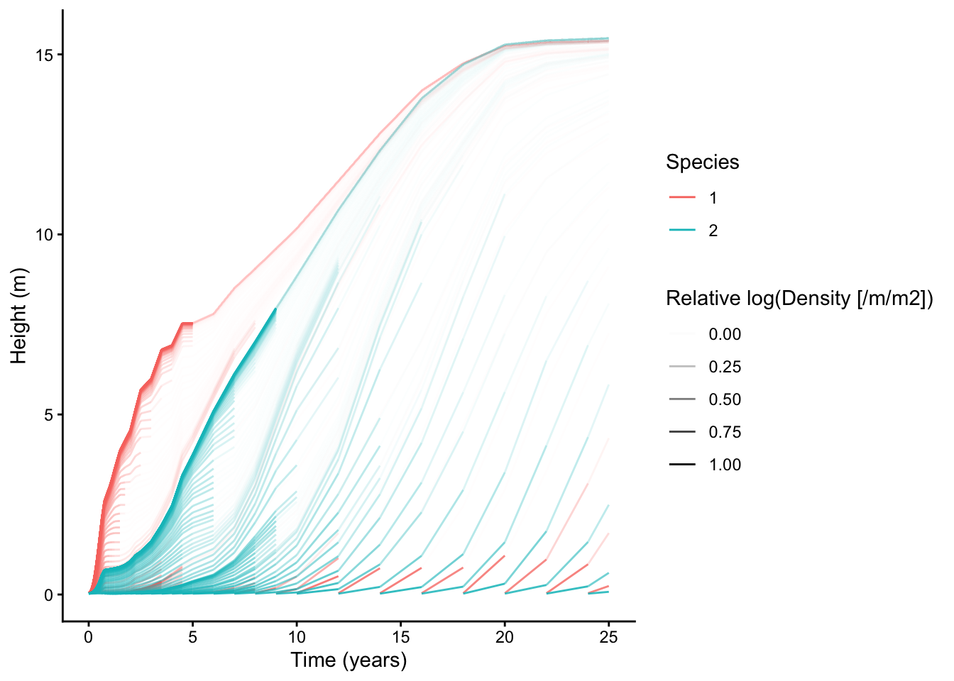
Calculate totals by species for each step
For each species, we can integrate over the height distribution to get the total value of the state variable per \(m^2\)
data_species_tot <-
  results_tidy$species %>% integrate_over_size_distribution()

data_species_tot
# A tibble: 202 × 24
step time patch_density species density min_height log_density height mortality fecundity area_heartwood mass_heartwood offspring_produced_survival_…¹ competition_effect height_inverse
<int> <dbl> <dbl> <chr> <dbl> <dbl> <dbl> <dbl> <dbl> <dbl> <dbl> <dbl> <dbl> <dbl> <dbl>
1 2 0.00001 0.140 1 0.0000999 0.0351 0.000310 0.00000351 0.0000000699 7.04e-31 5.59e-18 1.22e-16 7.04e-31 0.0000000261 0.00285
2 2 0.00001 0.140 2 0.0000999 0.0239 0.000437 0.00000239 0.0000000894 2.78e-31 2.59e-18 3.84e-17 2.78e-31 0.0000000121 0.00418
3 3 0.00002 0.140 1 0.000200 0.0351 0.000621 0.00000701 0.000000140 2.82e-30 2.24e-17 4.87e-16 2.82e-30 0.0000000522 0.00570
4 3 0.00002 0.140 2 0.000200 0.0239 0.000873 0.00000477 0.000000179 1.11e-30 1.04e-17 1.54e-16 1.11e-30 0.0000000242 0.00837
5 4 0.00003 0.140 1 0.000300 0.0351 0.000931 0.0000105 0.000000210 6.34e-30 5.03e-17 1.10e-15 6.33e-30 0.0000000784 0.00855
6 4 0.00003 0.140 2 0.000300 0.0239 0.00131 0.00000716 0.000000268 2.50e-30 2.33e-17 3.46e-16 2.50e-30 0.0000000363 0.0125
7 5 0.00004 0.140 1 0.000400 0.0351 0.00124 0.0000140 0.000000279 1.13e-29 8.95e-17 1.95e-15 1.13e-29 0.000000104 0.0114
8 5 0.00004 0.140 2 0.000400 0.0239 0.00175 0.00000955 0.000000357 4.45e-30 4.15e-17 6.15e-16 4.44e-30 0.0000000484 0.0167
9 6 0.00005 0.140 1 0.000500 0.0351 0.00155 0.0000175 0.000000349 1.76e-29 1.40e-16 3.04e-15 1.76e-29 0.000000131 0.0142
10 6 0.00005 0.140 2 0.000500 0.0239 0.00218 0.0000119 0.000000447 6.95e-30 6.48e-17 9.60e-16 6.95e-30 0.0000000605 0.0209
# ℹ 192 more rows
# ℹ abbreviated name: ¹offspring_produced_survival_weighted
# ℹ 9 more variables: net_mass_production_dt <dbl>, root_mass <dbl>, opt_psi_stem <dbl>, opt_root_psi <dbl>, transpiration <dbl>, E_up_ <dbl>, profit <dbl>, stom_cond_CO2 <dbl>, assimilation <dbl>For example, the number of individuals per \(m^2\) is found by integrating the density of each characteristic at a given step over height.
data_species_tot %>%
  ggplot(aes(time, density, colour=species)) +
  geom_line()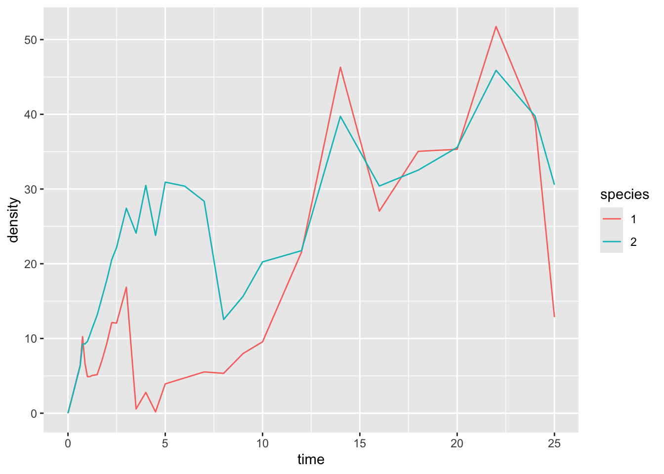
We can use the function TF24_expand_state to capture a large number of additional state variables (e.g.leaf area)
results_tidy_expand <- results_tidy %>% expand_state()

results_tidy_expand$species
# A tibble: 10,506 × 36
species time step patch_density node density log_density height mortality fecundity area_heartwood mass_heartwood offspring_produced_s…¹ competition_effect height_inverse net_mass_production_dt
<chr> <dbl> <int> <dbl> <int> <dbl> <dbl> <dbl> <dbl> <dbl> <dbl> <dbl> <dbl> <dbl> <dbl> <dbl>
1 1 0 1 0.140 1 22.3 3.11 0.0351 0.000699 0 0 0 0 0.000261 28.5 0.000988
2 1 1e-5 2 0.140 1 22.3 3.11 0.0351 0.000699 1.41e-26 1.12e-13 2.44e-12 1.41e-26 0.000261 28.5 0.000988
3 1 1e-5 2 0.140 2 22.3 3.11 0.0351 0.000699 0 0 0 0 0.000261 28.5 0.000988
4 1 2e-5 3 0.140 1 22.3 3.11 0.0351 0.000699 2.82e-26 2.24e-13 4.87e-12 2.82e-26 0.000261 28.5 0.000989
5 1 2e-5 3 0.140 2 22.3 3.11 0.0351 0.000699 1.41e-26 1.12e-13 2.44e-12 1.41e-26 0.000261 28.5 0.000988
6 1 2e-5 3 0.140 3 22.3 3.11 0.0351 0.000699 0 0 0 0 0.000261 28.5 0.000988
7 1 3e-5 4 0.140 1 22.3 3.11 0.0351 0.000699 4.23e-26 3.36e-13 7.31e-12 4.23e-26 0.000261 28.5 0.000989
8 1 3e-5 4 0.140 2 22.3 3.11 0.0351 0.000699 2.82e-26 2.24e-13 4.87e-12 2.82e-26 0.000261 28.5 0.000989
9 1 3e-5 4 0.140 3 22.3 3.11 0.0351 0.000699 1.41e-26 1.12e-13 2.44e-12 1.41e-26 0.000261 28.5 0.000988
10 1 3e-5 4 0.140 4 22.3 3.11 0.0351 0.000699 0 0 0 0 0.000261 28.5 0.000988
# ℹ 10,496 more rows
# ℹ abbreviated name: ¹offspring_produced_survival_weighted
# ℹ 20 more variables: root_mass <dbl>, opt_psi_stem <dbl>, opt_root_psi <dbl>, transpiration <dbl>, E_up_ <dbl>, profit <dbl>, stom_cond_CO2 <dbl>, assimilation <dbl>, area_leaf <dbl>,
# mass_leaf <dbl>, area_sapwood <dbl>, mass_sapwood <dbl>, area_bark <dbl>, mass_bark <dbl>, area_stem <dbl>, diameter_stem <dbl>, mass_root <dbl>, mass_live <dbl>, mass_total <dbl>,
# mass_above_ground <dbl>In the same way as individuals above, we can have a look at the total leaf area over time by intergrating across the size (i.e. height) distribution for a given step or time. This involves finding the product of the density of each of the characteristics present multiplied by the state variable in question (i.e. leaf area) before integrating across height.
data_species_tot <-
  results_tidy_expand$species %>%
  integrate_over_size_distribution()

data_species_tot %>%
  ggplot(aes(time, area_leaf, colour = species)) +
  geom_line()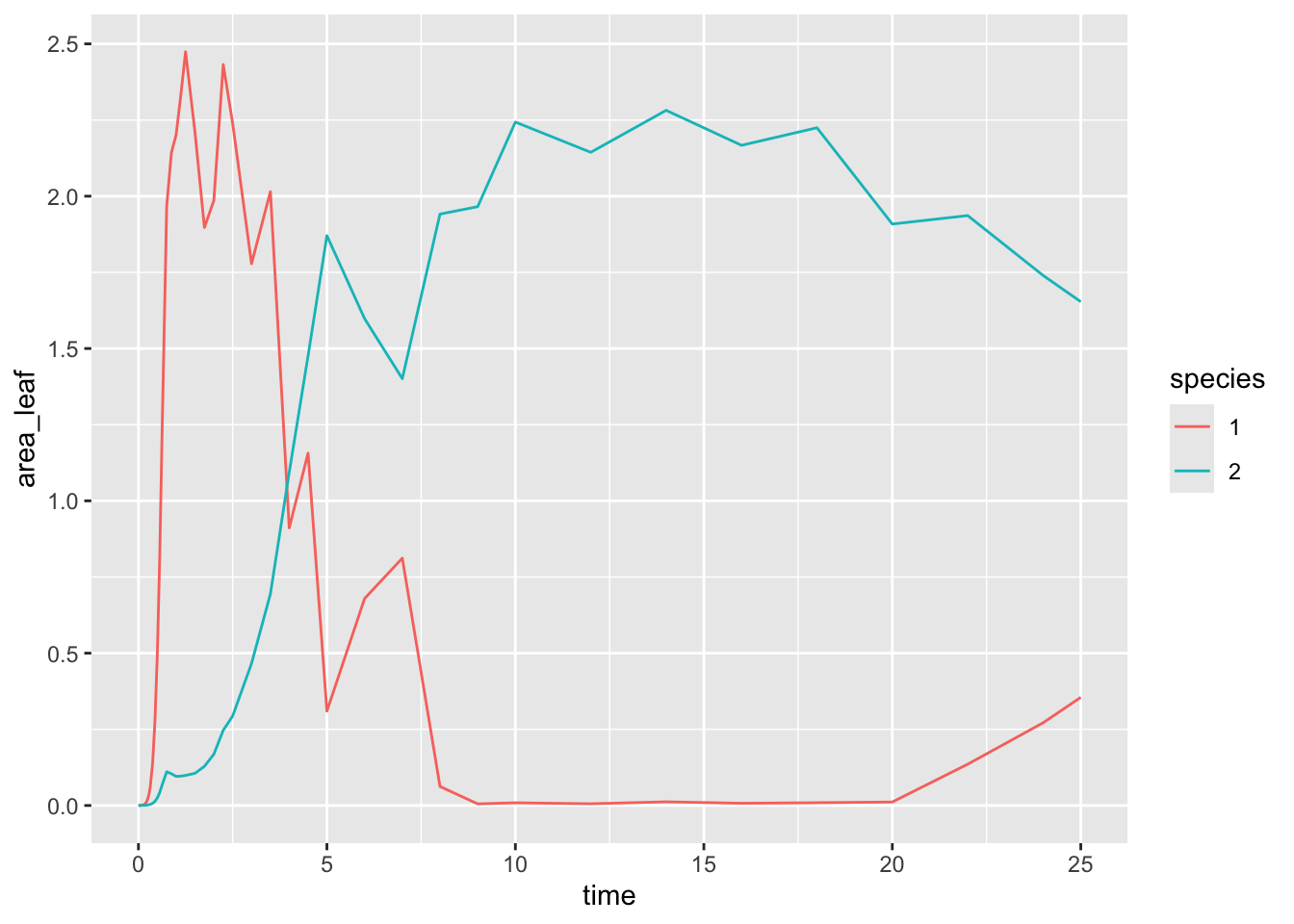
In this case, species 1 with cheap, thin leaves briefly has a much higher total leaf area deployed comapred across the height distribution before eventually being overtaken by species with thicker, more expensive leaves.
We can convert these integrated total state variables into their respective biomass components to get an idea of how total biomass and relative biomass allocation varies through time for each species.
v <- c("mass_heartwood", "mass_sapwood", "mass_bark", "mass_leaf")

data_long <-
  data_species_tot %>%
  select(time,species, one_of(v)) %>%
  pivot_longer(cols=starts_with("mass"), names_to = "tissue")

data_long$tissue <- factor(data_long$tissue, levels = v)

species_names <- tibble(species = unique(data_long$species),
                      species_name = c("Species_1","Species_2"))

data_long %>%
  left_join(species_names) %>%
  ggplot(aes(time, value, fill=tissue)) +
  geom_area() +
  labs(x = "Patch age (yr)", y = "Above ground mass (kg/m2)") +
  theme_classic() +
  xlim(c(0,100)) +
  facet_wrap(~species_name)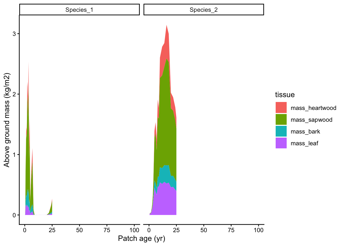
Interpolate to specific times
The node-spacing algorithm determines the optimum introduction times for the characteristics, which means that the time values associated with steps may not correspond to known times that we might like to extract information about. For example, what the total amount of biomass per \(m^2\) will be at 50 years. By doing this, it also means that we can integrate between defined times. Let’s work with our results again by running a patch again and then tidying.
results <- run_mypatch(traits =  trait_matrix(c(0.07, 0.24), c("lma")))

results_tidy <- results
Lets interpolate our results from the run_mypatch above for timepoints 1,5,10 using the function interpolate_to_times. Note that time in units of years.
times <- c(1, 5, 10)

tidy_species_data <- results_tidy$species

tidy_species_new <- interpolate_to_times(tidy_species_data, times)
Gives interpolated values for state variables at new time points.
tidy_species_new %>% drop_na()# A tibble: 493 × 23
species node time patch_density density log_density height mortality fecundity area_heartwood mass_heartwood offspring_produced_surv…¹ competition_effect height_inverse net_mass_production_dt
<chr> <int> <dbl> <dbl> <dbl> <dbl> <dbl> <dbl> <dbl> <dbl> <dbl> <dbl> <dbl> <dbl> <dbl>
1 1 1 1 0.138 1.42e+ 0 0.351 3.36 0.0107 -4.83e-13 0.0000382 0.0653 2.85e-14 2.40 0.297 2.97
2 1 1 5 0.0953 1.48e- 1 -5.27 10.2 4.37 1.98e- 3 0.00220 11.4 1.01e- 3 21.9 0.0984 13.7
3 1 1 10 0.0298 -8.90e-10 -589549. 14.2 589549. 2.67e+ 3 0.00673 46.8 6.82e- 2 42.8 0.0705 -3.39
4 1 2 1 0.138 1.42e+ 0 0.351 3.36 0.0107 -4.83e-13 0.0000382 0.0653 2.85e-14 2.40 0.297 2.97
5 1 2 5 0.0953 1.51e- 1 -5.24 10.2 4.37 1.98e- 3 0.00220 11.4 1.01e- 3 21.9 0.0984 13.7
6 1 2 10 0.0298 -9.19e-10 -589373. 14.2 589374. 2.67e+ 3 0.00673 46.8 6.83e- 2 42.8 0.0705 -3.39
7 1 3 1 0.138 1.42e+ 0 0.351 3.36 0.0107 -4.83e-13 0.0000382 0.0653 2.85e-14 2.40 0.297 2.97
8 1 3 5 0.0953 1.49e- 1 -5.25 10.2 4.37 1.98e- 3 0.00220 11.4 1.01e- 3 21.9 0.0984 13.7
9 1 3 10 0.0298 -9.09e-10 -589198. 14.2 589198. 2.67e+ 3 0.00673 46.8 6.83e- 2 42.8 0.0705 -3.39
10 1 4 1 0.138 1.42e+ 0 0.351 3.36 0.0107 -4.83e-13 0.0000382 0.0653 2.85e-14 2.40 0.297 2.97
# ℹ 483 more rows
# ℹ abbreviated name: ¹offspring_produced_survival_weighted
# ℹ 8 more variables: root_mass <dbl>, opt_psi_stem <dbl>, opt_root_psi <dbl>, transpiration <dbl>, E_up_ <dbl>, profit <dbl>, stom_cond_CO2 <dbl>, assimilation <dbl>We can now assess their correspondence with the values already predicted in the original results output. We can see in this case that the points (represneting the interpolated values) fall along the curves which indicates good correspondence bewteen our interpolation and the original simulation.
data_combined <-
  tidy_species_data %>%
  bind_rows(tidy_species_new) %>%
  arrange(species, node, time) %>%
  filter(node %in% seq(1, 101, by=20))

data_combined_long <-
  data_combined  %>%
  select(node, time, step, density, height, species) %>%
  pivot_longer(cols = c("density", "height"))

data_combined_long %>%
  ggplot(aes(time, value, group=node,colour=node)) +
  geom_line() +
  geom_point(data = data_combined_long %>% filter(is.na(step)), col=2) +
  scale_y_log10() +
  xlim(c(0, 20)) +
  facet_grid(name~species, scales="free") +
  theme_classic()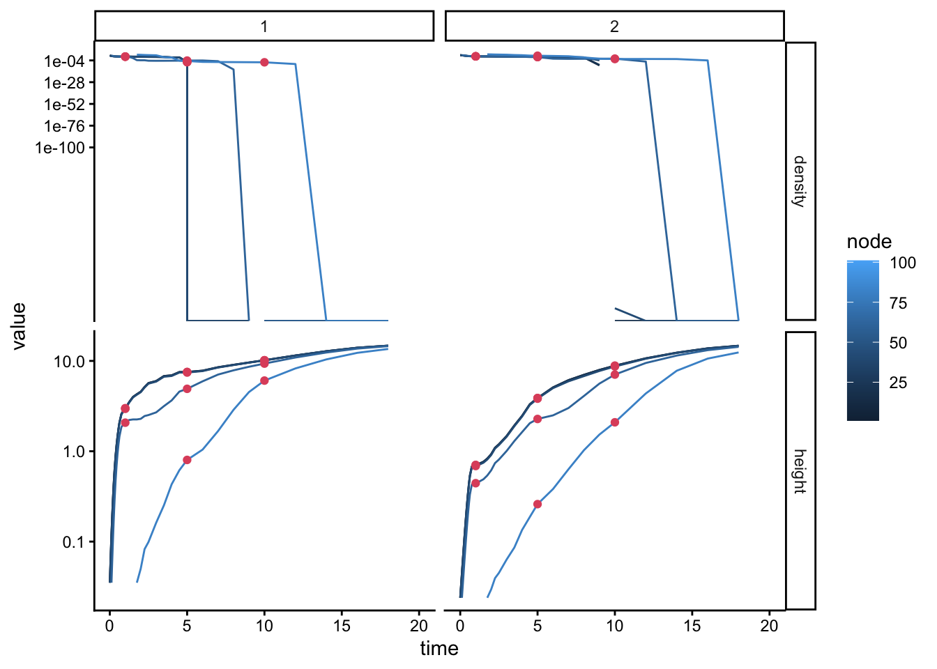
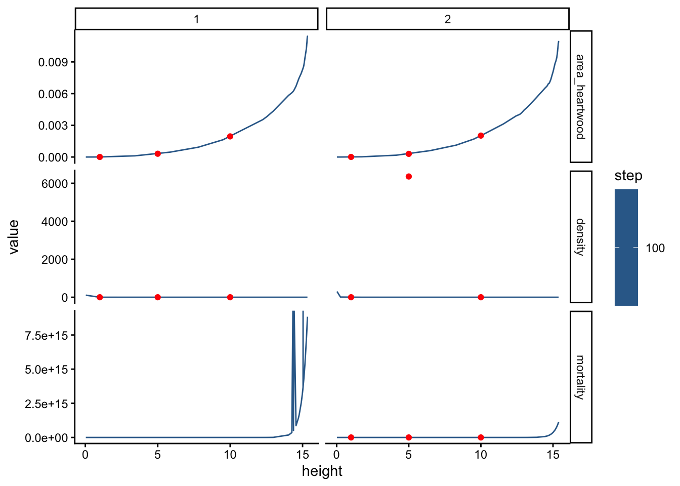
Interpolate to specific heights
Similar to above, we can interpolate across nodes at given time to sepcific heights, using the function interpolate_to_heights
heights <- c(1, 5, 10)

tidy_species_data <- results_tidy$species

tidy_species_new <- interpolate_to_heights(tidy_species_data, heights)
Gives predictions at new height.
tidy_species_new %>% drop_na()# A tibble: 229 × 23
species time step patch_density density log_density height mortality fecundity area_heartwood mass_heartwood offspring_produced_surv…¹ competition_effect height_inverse net_mass_production_dt
<chr> <dbl> <int> <dbl> <dbl> <dbl> <dbl> <dbl> <dbl> <dbl> <dbl> <dbl> <dbl> <dbl> <dbl>
1 1 0 1 0.140 22.3 3.11 0.0351 0.000699 0 0 0 0 0.000261 28.5 0.000988
2 1 0.00001 2 0.140 22.3 3.11 0.0351 0.000699 1.41e-26 1.12e-13 2.44e-12 1.41e-26 0.000261 28.5 0.000988
3 1 0.00002 3 0.140 22.3 3.11 0.0351 0.000699 2.82e-26 2.24e-13 4.87e-12 2.82e-26 0.000261 28.5 0.000989
4 1 0.00003 4 0.140 22.3 3.11 0.0351 0.000699 4.23e-26 3.36e-13 7.31e-12 4.23e-26 0.000261 28.5 0.000989
5 1 0.00004 5 0.140 22.3 3.11 0.0351 0.000699 5.64e-26 4.48e-13 9.75e-12 5.64e-26 0.000262 28.5 0.000989
6 1 0.00005 6 0.140 22.3 3.11 0.0351 0.000700 7.05e-26 5.60e-13 1.22e-11 7.05e-26 0.000262 28.5 0.000990
7 1 0.00006 7 0.140 22.3 3.11 0.0351 0.000700 8.46e-26 6.72e-13 1.46e-11 8.46e-26 0.000262 28.5 0.000990
8 1 0.00007 8 0.140 22.3 3.10 0.0351 0.000700 9.88e-26 7.84e-13 1.71e-11 9.87e-26 0.000262 28.5 0.000990
9 1 0.00008 9 0.140 22.3 3.10 0.0351 0.000700 1.13e-25 8.96e-13 1.95e-11 1.13e-25 0.000262 28.5 0.000991
10 1 0.0000953 10 0.140 22.3 3.10 0.0351 0.000700 1.34e-25 1.07e-12 2.32e-11 1.34e-25 0.000262 28.5 0.000991
# ℹ 219 more rows
# ℹ abbreviated name: ¹offspring_produced_survival_weighted
# ℹ 8 more variables: root_mass <dbl>, opt_psi_stem <dbl>, opt_root_psi <dbl>, transpiration <dbl>, E_up_ <dbl>, profit <dbl>, stom_cond_CO2 <dbl>, assimilation <dbl>To see how good these are, plot together with old points
data_combined <-
  tidy_species_data %>%
  bind_rows(tidy_species_new) %>%
  arrange(species, time, height) %>%
  filter(step %in% c(100, 142))

data_combined_long <-
  data_combined  %>%
  select(node, time, step, height, density, mortality, area_heartwood, species) %>%
  pivot_longer(cols = c("density", "mortality", "area_heartwood"))

data_combined_long %>%
    filter(!is.na(node)) %>%
  ggplot() +
  geom_line(aes(height, value, group=step, colour=step)) +
  geom_point(data = data_combined_long %>% filter(is.na(node)), aes(x=height, y=value), col="red")+
  facet_grid(name~species, scales="free") +
  theme_classic()