library(plant)
library(dplyr)
library(tidyr)
library(ggplot2)

base <- function(type) {
  scm_base_parameters(type) |>
    add_strategies(trait_matrix(0.0825, "lma"), birth_rate = 20)
}TF24: hydraulics, and a fast acclimating variant
guide
TF24 represents the movement of water from soil, through roots and stems, to leaves. At each rate calculation it finds the root-collar water potential that best balances two outcomes: opening stomata increases photosynthesis, but more negative water potential increases hydraulic risk.
The standard TF24 model solves this optimisation from scratch each time. TF24f (“f” for fast or forecasting) instead carries the operating point forward and allows it to adjust as conditions change. In practical terms, TF24 repeatedly finds the optimum, whereas TF24f tracks it.
Tracking can reduce repeated calculations and also introduces a finite acclimation time. This guide explains that approximation, compares the two models, and shows the parameter that controls tracking speed.
The idea: let the optimum chase a moving target
As a plant grows and its environment changes, the preferred operating point moves. TF24f stores its current estimate as an extra state variable and adjusts that state in the direction that increases carbon profit:
\[\frac{\mathrm{d}\psi}{\mathrm{d}t} = k \,\frac{\partial\,\text{profit}}{\partial\psi}.\]
At the optimum, the profit gradient is zero and the state stops moving. When the optimum shifts, the gradient moves the state towards its new value. The gain \(k\) controls how quickly that adjustment occurs and therefore how much acclimation lag remains.
NoteHow the gradient is calculated
By default, plant calculates the gradient exactly with automatic differentiation and the implicit-function theorem (use_ad_gradient = TRUE). A centred finite-difference calculation is available as a fallback. In R, k_acclim controls the gain, use_ad_gradient selects the method, and psi_fd_step matters only on the finite-difference path.
Run TF24 and TF24f side by side
The following example gives both models the same trait and recruitment inputs. For TF24f we use an illustrative gain of 2; the package default is 1.
tf24  <- run_scm(base("TF24"),  collect = TRUE, refine_schedule = FALSE)

p_f <- base("TF24f")
s <- p_f$strategies[[1]]
s$k_acclim <- 2
s$use_ad_gradient <- TRUE
p_f$strategies[[1]] <- s
tf24f <- run_scm(p_f, collect = TRUE, refine_schedule = FALSE)
In this example, the two size structures remain very similar:
bind_rows(
  tf24$species  |> drop_na() |> mutate(model = "TF24 (optimised)"),
  tf24f$species |> drop_na() |> mutate(model = "TF24f (tracked)")
) |>
  plot_size_distribution() +
  facet_wrap(~model) +
  coord_cartesian(expand = FALSE) +
  labs(title = "Same biology, two ways of resolving the leaf optimum")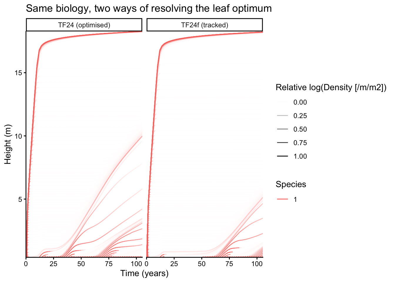
TF24f records the tracked potential in opt_root_psi_state. TF24 reports its newly optimised value as opt_root_psi, with the opposite sign convention in this output. Plotting them together reveals the acclimation lag: early in life, the optimum moves faster than the finite-gain state can follow. The gap then narrows as growth slows.
node1 <- function(d) d |> filter(node == 1) |> drop_na()
bind_rows(
  node1(tf24$species)  |> transmute(time, psi = -opt_root_psi,       model = "TF24 optimum"),
  node1(tf24f$species) |> transmute(time, psi = opt_root_psi_state, model = "TF24f tracked")
) |>
  ggplot(aes(time, psi, colour = model)) +
  geom_line() +
  labs(x = "Patch age (years)", y = "Root-collar potential (MPa)",
       colour = NULL, title = "The tracked state follows the moving optimum") +
  theme_classic()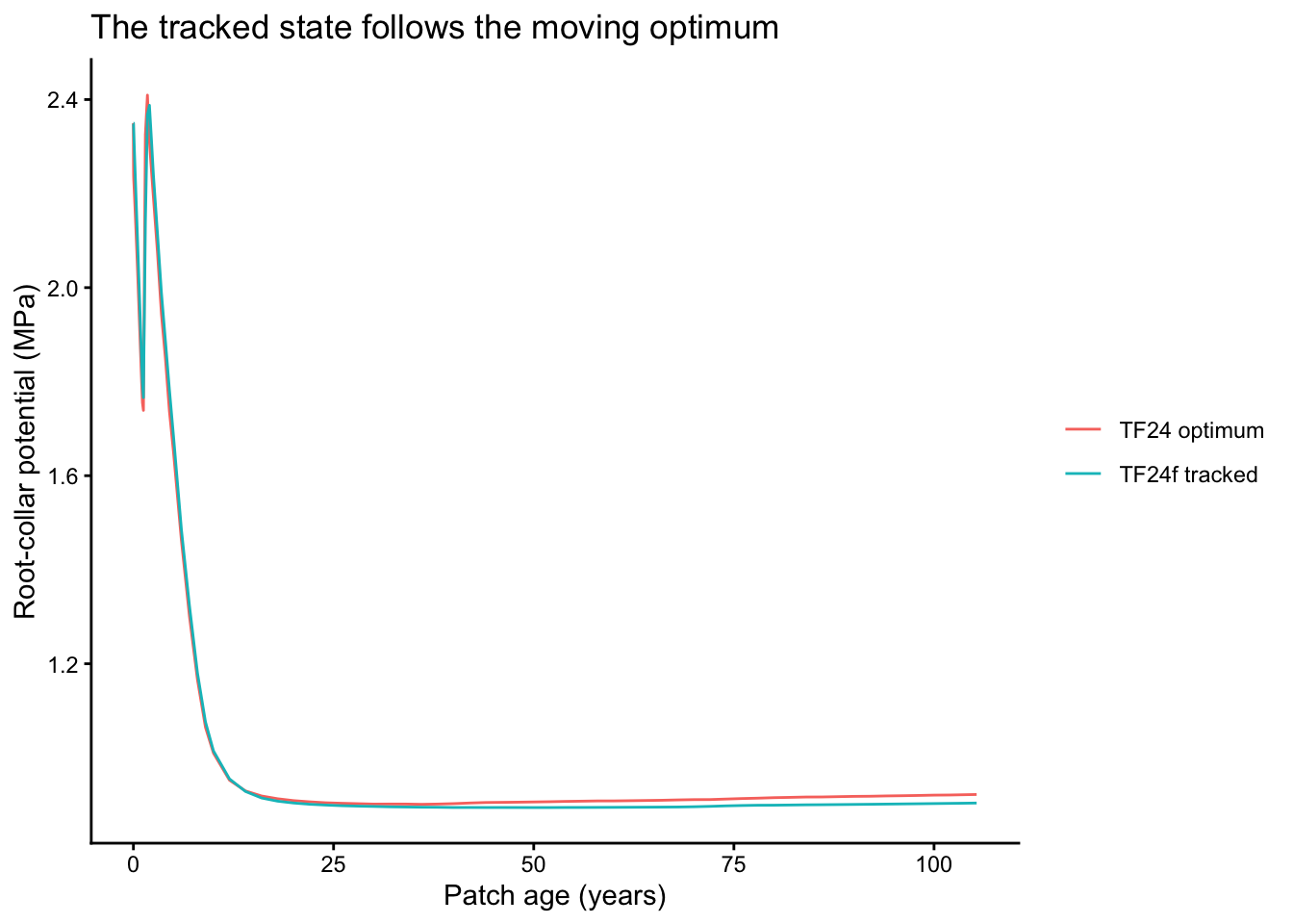
Choosing the gain k
A larger k makes the tracked state respond more quickly, but it also makes the extra ODE state stiffer, which can force the adaptive solver to take many smaller steps. A smaller k is easier to integrate but produces a longer acclimation lag. There is therefore no universal best value: compare TF24f against TF24 over the environmental range and time scale relevant to the analysis.
The default automatic-differentiation path avoids a finite-difference step and its truncation error. If use_ad_gradient = FALSE, TF24f instead uses a centred finite difference controlled by psi_fd_step; that fallback should be treated as a numerical sensitivity setting and checked explicitly.
A note on initialisation
Each new seedling starts with its tracked state at the current optimum. Without this initial full solve, a seedling would begin at a non-physical value and could temporarily escape the light limitation that should suppress it. After initialisation, TF24f resumes tracking rather than re-optimising at every step.
Status
TF24f currently tracks root-collar potential and inherits TF24’s selectable canopy models. It is an approximation with an explicit acclimation lag, not an exact replacement for TF24.