Case study 3: Canham function growth with tree data from Barro Colorado Island
Source:vignettes/canham.Rmd
canham.Rmd
library(hmde)
library(dplyr)
#>
#> Attaching package: 'dplyr'
#> The following objects are masked from 'package:stats':
#>
#>     filter, lag
#> The following objects are masked from 'package:base':
#>
#>     intersect, setdiff, setequal, union
library(ggplot2)
Our final case study reproduces analysis from O’Brien et al. (2024) with a small sample size for G. recondita in order to make the model tractable for a demonstration.
The function we use here is based on Canham et al. (2004), and is a three parameter non-linear ODE given by The Canham function, as we refer to it, describes hum-shaped growth that accelerates to a peak at then declines to 0 at a rate controlled by . The Canham function does not have an analytic solution the way that the previous function did, so we are unable to directly encode the sizes over time and must instead use a numerical method.
The Canham function has been used for a lot of growth analysis such as Herault et al. (2011) and Canham et al. (2006) as well as our own previous work in O’Brien et al. (2024) and [Paper 2]. The desirable features of the Canham growth model are that it has a period of increasing growth at small sizes, with a finite growth peak at , and then decay to near-zero growth. With different parameter combinations Canham can fit a range of growth behaviours to an observed interval: increasing growth, decreasing growth, a growth spike, or steady growth. The downside is that the Canham function is unimodal – it can only fit a single peak and as such is not suitable to describe the full life history of species that are strongly responsive to their environment as seen in [Paper 2].
The next bit of code plots the Canham function for chosen parameter values. We have provided some, but encourage playing around with the parameters and seeing what happens to the function.
g_max <- 1 #Max growth rate
S_max <- 10 #Size at which the maximum growth occurs
k <- 0.75
y_0 <- 1 #Starting size
y_final <- 40

#Plot of growth function
ggplot() +
  xlim(y_0, y_final) +
  labs(x = "Y(t)", y = "f", title = "Canham growth") +
  theme_classic() +
  theme(axis.text=element_text(size=16),
        axis.title=element_text(size=18,face="bold")) +
  geom_function(fun=hmde_model_des("canham_single_ind"),
                args=list(pars = list(g_max, S_max, k)),
                colour="green4", linewidth=1,
                xlim=c(y_0, y_final))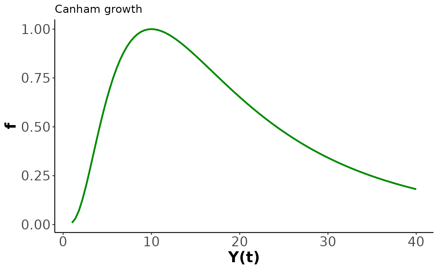
The default priors for the Canham top-level parameters for the single
individual model are
For the multi-individual model the prior structure and default
parameters are
To see the name for the prior parameter run hmde_model. For
example in the following we want to change the prior for
(ind_max_growth) in the individual model:
prior_pars(hmde_model("canham_single_ind"))
#> $prior_pars_ind_max_growth
#> [1] 0 2
#>
#> $prior_pars_ind_size_at_max_growth
#> [1] 0 2
#>
#> $prior_pars_ind_k
#> [1] 0 2
#>
#> $prior_pars_global_error_sigma
#> [1] 0 2
#prior_pars_ind_max_growth is the argument name for the prior parametersAs some exploratory analysis we’re going to look at the size and growth increment distributions.
hist(Tree_Size_Data$y_obs,
     xlab = "Size (cm)", main ="")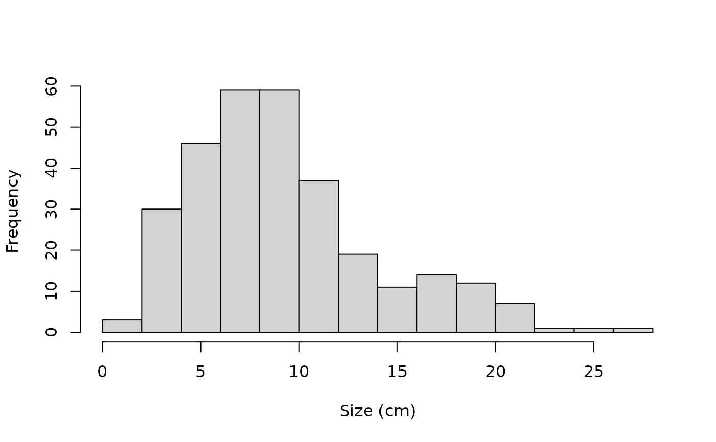
Tree_Size_Data_Transformed <- Tree_Size_Data %>%
  group_by(ind_id) %>%
  mutate(Delta_y_obs = y_obs - lag(y_obs)) %>%
  ungroup() %>%
  arrange(ind_id, time) %>%
  filter(!is.na(Delta_y_obs))

hist(Tree_Size_Data_Transformed$Delta_y_obs,
     xlab = "Growth increment (cm)", main="")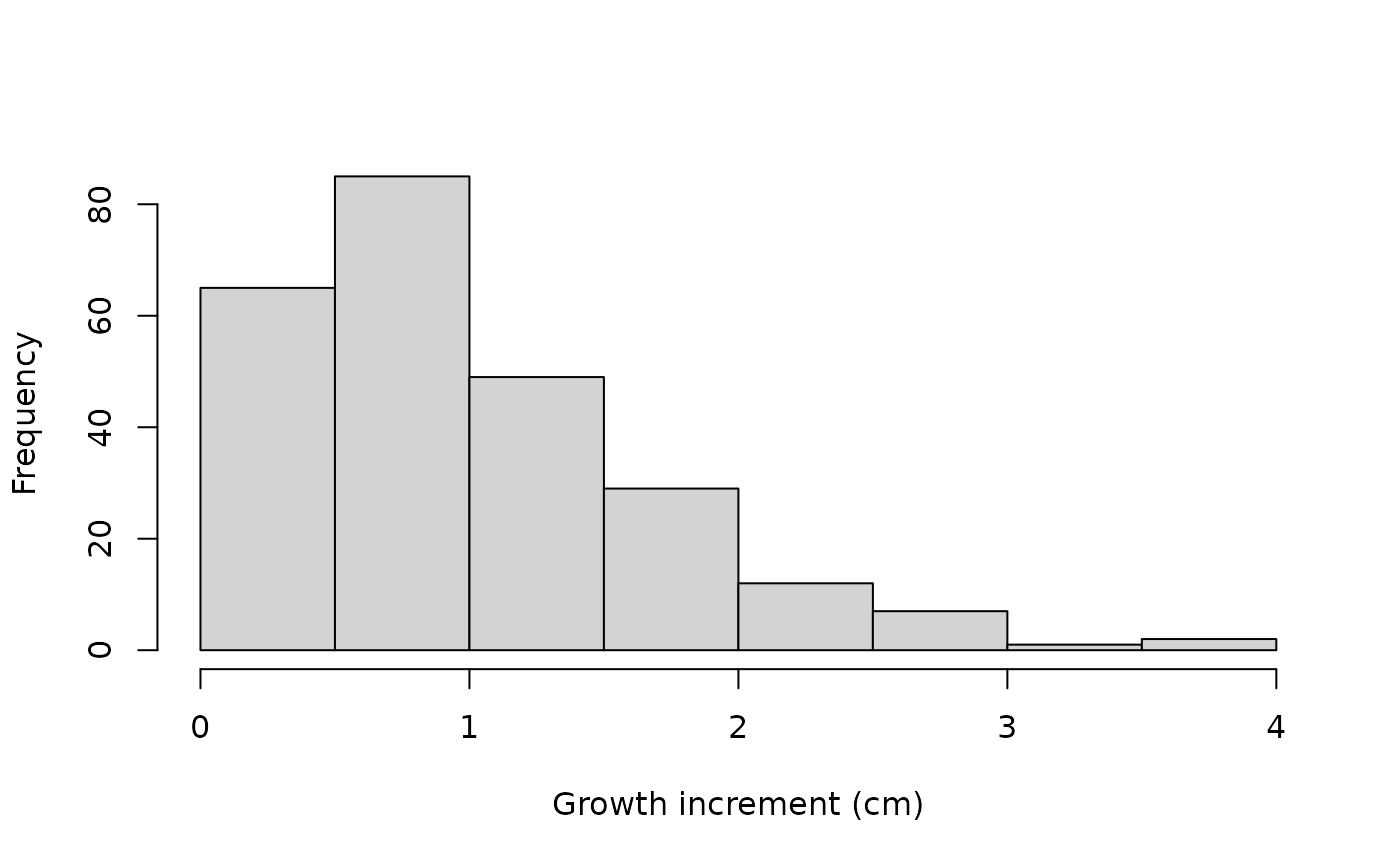
Due to the complexity of the Canham model the sampling can take up to
3 hours. If you decide to run your own samples we recommend saving the
model outputs using saveRDS() so you don’t need to rerun
your model every time. We provide a data set of estimates with the
package in the Tree_Size_Ests data file which can be
accessed directly.
set.seed(2026)
tree_canham_fit <- hmde_data_template("canham_multi_ind",
                                      obs_data = Tree_Size_Data) |>
  hmde_run(chains = 4, cores = 4, iter = 2000)

tree_canham_estimates <- hmde_estimates(fit = tree_canham_fit,
                                 obs_data = Tree_Size_Data)

saveRDS(tree_canham_fit, "tree_canham_fit.rds")
#saveRDS(tree_canham_estimates, "tree_canham_estimates.rds")
The model analysis follows the same workflow as the previous demonstrations: we look at how individual sizes over time and fitted growth functions behave, then examine evidence of relationships between parameter values at the individual level. We also look at the species-level parameter CIs and estimates.
measurement_data_transformed <- measurement_ests(Tree_Size_Ests) %>%
  group_by(ind_id) %>%
  mutate(
    delta_y_obs = y_obs - lag(y_obs),
    obs_interval = time - lag(time),
    obs_growth_rate = delta_y_obs/obs_interval,
    delta_y_est = y_hat - lag(y_hat),
    est_growth_rate = delta_y_est/obs_interval
  ) %>%
  ungroup()

#Distributions of estimated growth and size
ggplot(measurement_data_transformed,
       aes(y_hat)) +
  geom_histogram(bins = 10,
                 colour = "black",
                 fill = "lightblue") +
  labs(x="Size (cm)",
       title = "Estimated size distribution") +
  theme_classic()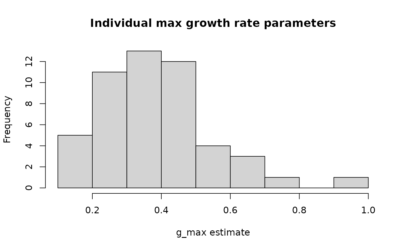
ggplot(measurement_data_transformed,
       aes(delta_y_est)) +
  geom_histogram(bins = 10,
                 colour = "black",
                 fill = "lightblue") +
  labs(x = "Growth increment (cm)",
       title = "Estimated growth increments") +
  theme_classic()
#> Warning: Removed 50 rows containing non-finite outside the scale range
#> (`stat_bin()`).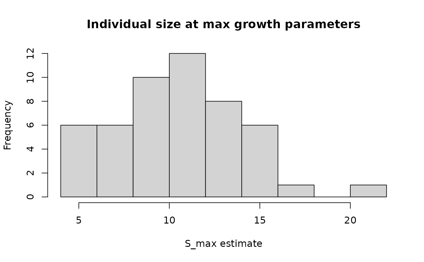
ggplot(measurement_data_transformed,
       aes(est_growth_rate)) +
  geom_histogram(bins = 10,
                 colour = "black",
                 fill = "lightblue") +
  labs(x = "Growth rate (cm/yr)",
       title = "Estimated annualised growth rate distribution") +
  theme_classic()
#> Warning: Removed 50 rows containing non-finite outside the scale range
#> (`stat_bin()`).
#Quantitative R^2
cor(measurement_data_transformed$y_obs, measurement_data_transformed$y_hat)^2
#> [1] 0.9968881

r_sq_est <- cor(measurement_ests(Tree_Size_Ests)$y_obs,
                measurement_ests(Tree_Size_Ests)$y_hat)^2
r_sq <- paste0("R^2 = ",
               signif(r_sq_est,
                      digits = 3))

obs_est_scatter <- ggplot(data = measurement_ests(Tree_Size_Ests),
       aes(x = y_obs, y = y_hat)) +
  geom_point(shape = 16, size = 1, colour = "green4") +
  xlab("Y obs.") +
  ylab("Y est.") +
  geom_abline(slope = 1, linetype = "dashed") +
  annotate("text", x = 7, y = 22,
           label = r_sq) +
  theme_classic()
obs_est_scatter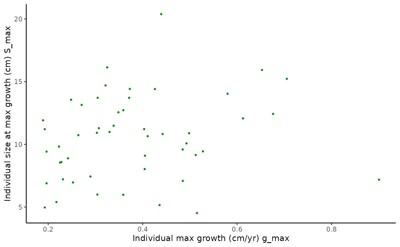
#Plots of size over time for a sample of 5 individuals
obs_est_size_plot <- hmde_plot_obs_est_inds(estimates = Tree_Size_Ests,
                                            n_ind_to_plot = 5) +
  theme(legend.position = "inside",
        legend.position.inside = c(0.1, 0.85)) +
  guides(colour=guide_legend(nrow=2,byrow=TRUE))
obs_est_size_plot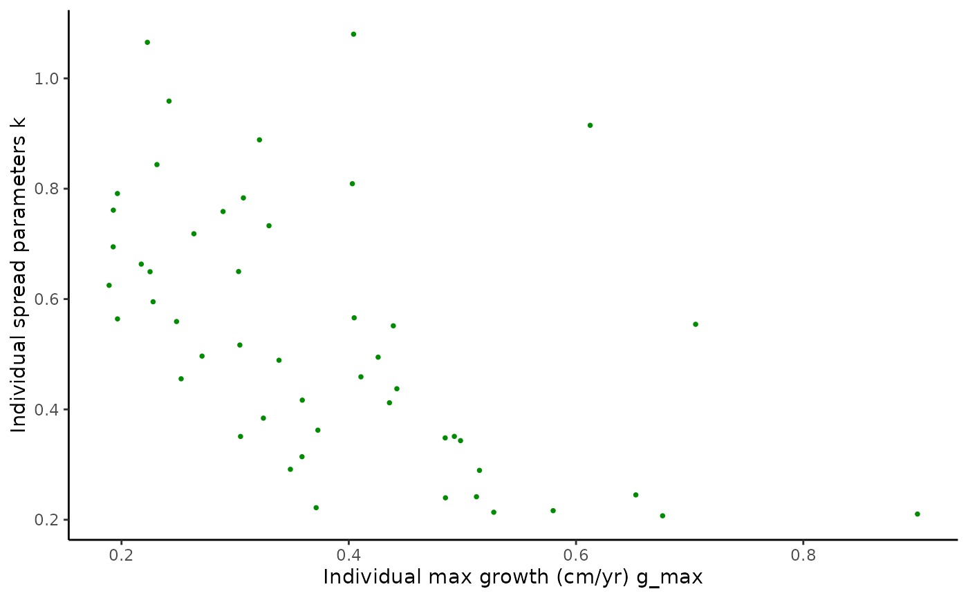
Individual parameter analysis, growth function plots follow this.
#1-dimensional parameter distributions
ggplot(individual_ests(Tree_Size_Ests),
       aes(ind_max_growth_mean)) +
  geom_histogram(bins = 10,
                 colour = "black",
                 fill = "lightblue") +
  labs(x="g_max estimate") +
  theme_classic()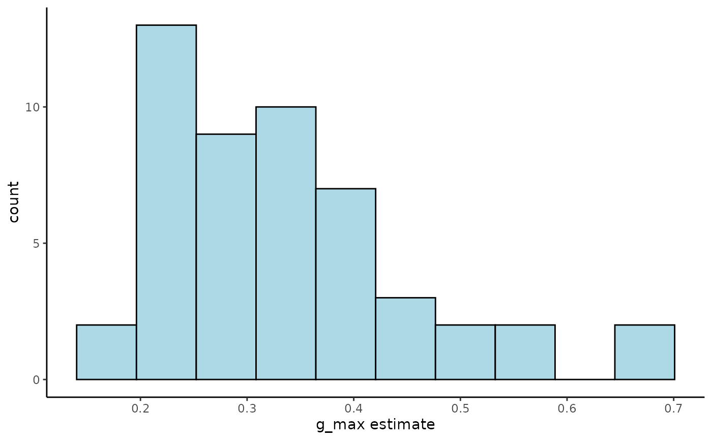
ggplot(individual_ests(Tree_Size_Ests),
       aes(ind_size_at_max_growth_mean)) +
  geom_histogram(bins = 10,
                 colour = "black",
                 fill = "lightblue") +
  labs(x="S_max estimate") +
  theme_classic()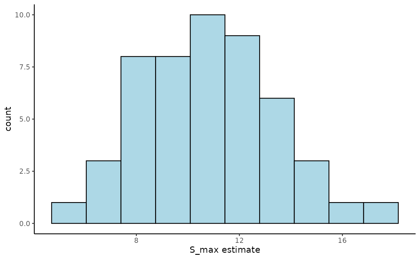
ggplot(individual_ests(Tree_Size_Ests),
       aes(ind_k_mean)) +
  geom_histogram(bins = 10,
                 colour = "black",
                 fill = "lightblue") +
  labs(x="k estimate") +
  theme_classic()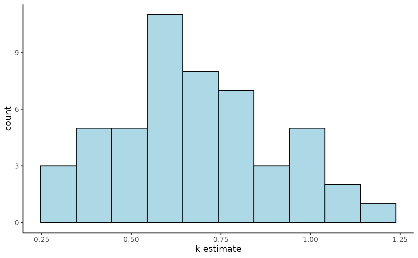
#2-dimensional parameter distributions
pairplot1 <- ggplot(data = individual_ests(Tree_Size_Ests),
       aes(x = ind_max_growth_mean, y = ind_size_at_max_growth_mean)) +
  geom_point(shape = 16, size = 1, colour = "green4") +
  xlab("Ind. max growth (cm/yr)") +
  ylab("Ind. size at max growth (cm)") +
  theme_classic()

pairplot2 <- ggplot(data = individual_ests(Tree_Size_Ests),
       aes(x = ind_max_growth_mean, y = ind_k_mean)) +
  geom_point(shape = 16, size = 1, colour = "green4") +
  xlab("Ind. max growth (cm/yr)") +
  ylab("Ind. spread par.") +
  theme_classic()

pairplot3 <- ggplot(data = individual_ests(Tree_Size_Ests),
       aes(x = ind_k_mean, y = ind_size_at_max_growth_mean)) +
  geom_point(shape = 16, size = 1, colour = "green4") +
  xlab("Ind. spread par.") +
  ylab("Ind. size at max growth (cm)") +
  theme_classic()

pairplot1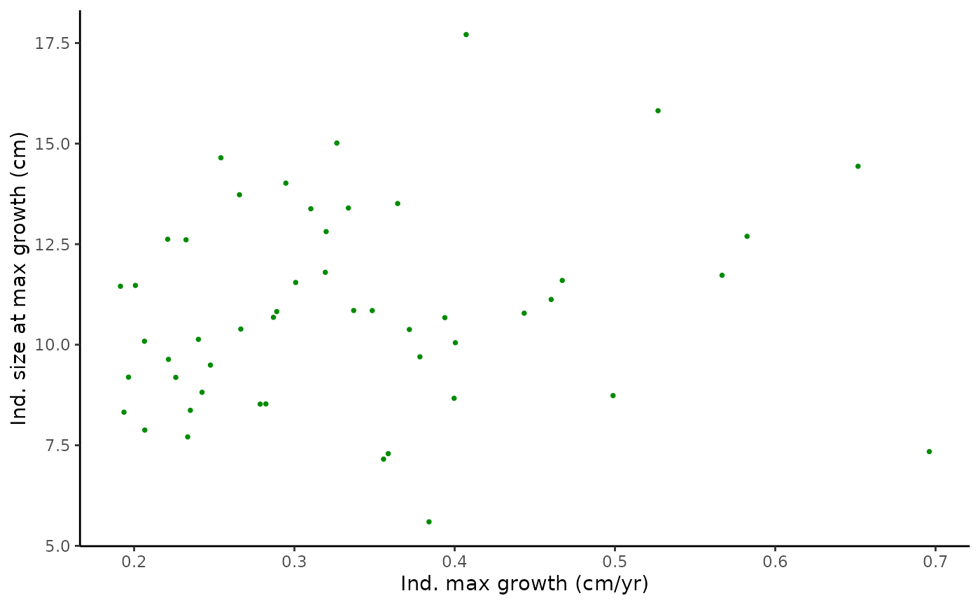
pairplot2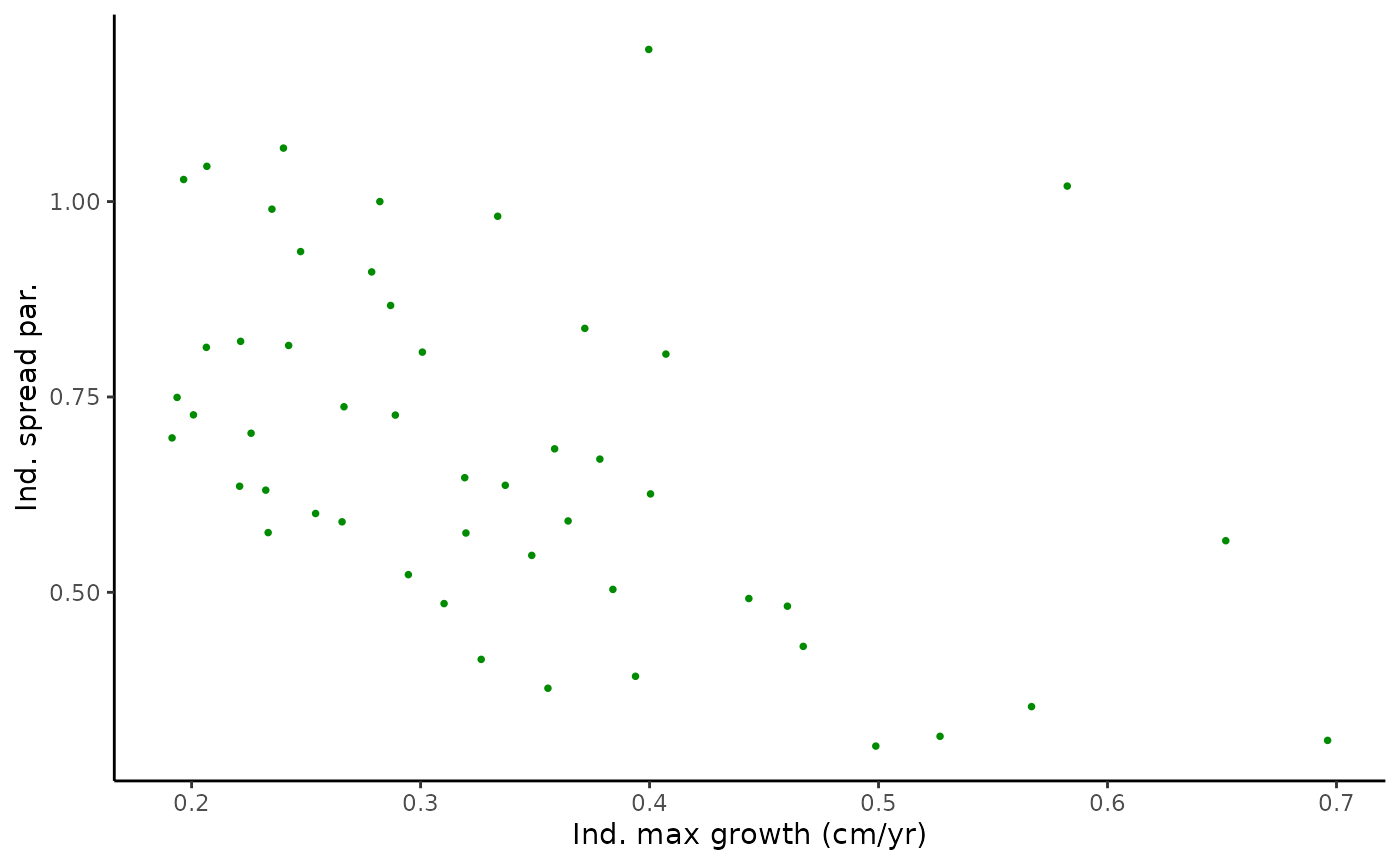
pairplot3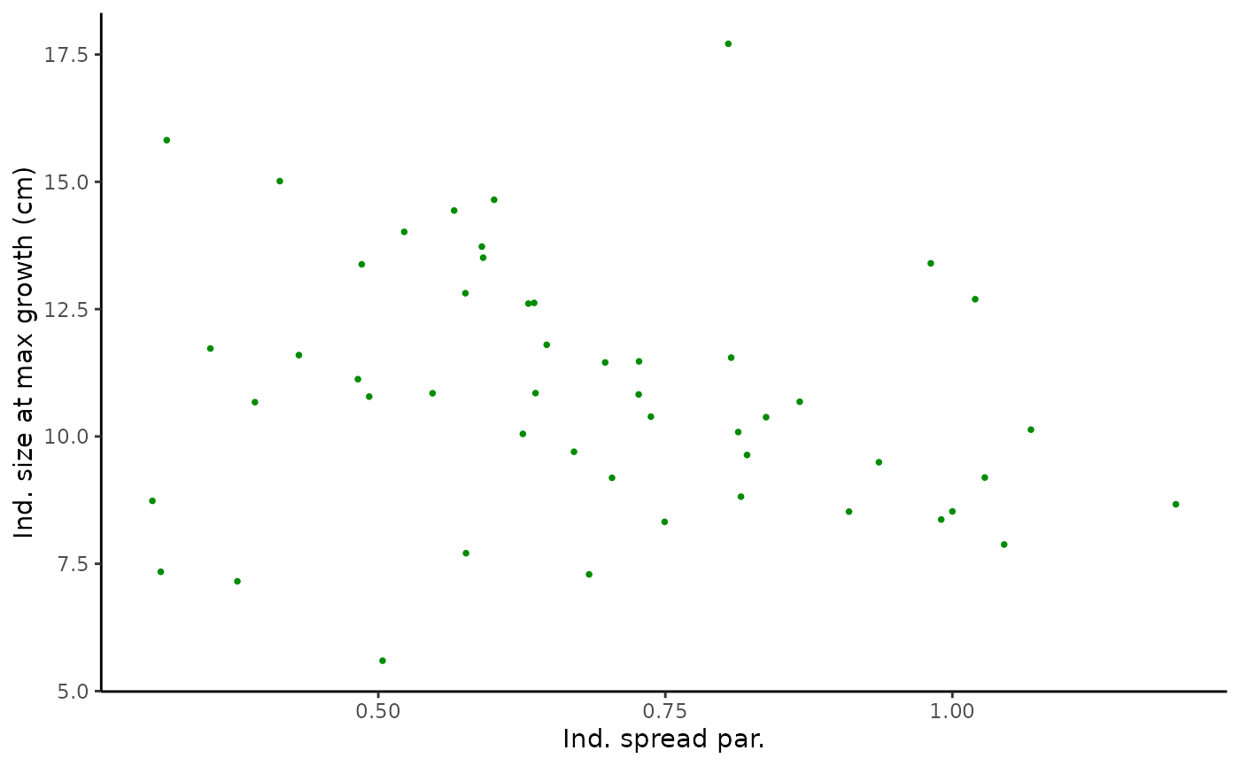
#monotonic correlation of parameters
cor(individual_ests(Tree_Size_Ests)[,c(2,6,10)], method="spearman")
#>                             ind_max_growth_mean ind_size_at_max_growth_mean
#> ind_max_growth_mean                   1.0000000                 -0.40081633
#> ind_size_at_max_growth_mean          -0.4008163                  1.00000000
#> ind_k_mean                           -0.3939016                 -0.01310924
#>                              ind_k_mean
#> ind_max_growth_mean         -0.39390156
#> ind_size_at_max_growth_mean -0.01310924
#> ind_k_mean                   1.00000000

#Plot function pieces over estimated sizes.
est_de_plot <- hmde_plot_de_pieces(Tree_Size_Ests)
est_de_plot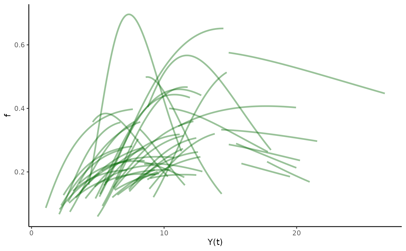
At the hyper-parameter level for the whole population we have centre and spread parameters for the log-normal distributions of , and .
pars_CI_names <- c(
  "mean log max growth rate",
  "mean max growth rate in cm/yr",
  "log max growth rate standard deviation",
  "mean log size at max growth rate",
  "mean max size at max growth rate in cm",
  "log max size at growth rate standard deviation",
  "mean mean log spread parameter",
  "mean mean spread parameter",
  "log spread parameter standard deviation"
)

#Vector that picks out which pars to be exponentiated
exp_vec <- c(FALSE, TRUE, FALSE,
             FALSE, TRUE, FALSE,
             FALSE, TRUE, FALSE)

#Print mean estimates and CIs
for(i in 1:nrow(population_ests(Tree_Size_Ests))){
  if(!exp_vec[i]){
    print(paste0(pars_CI_names[i],
                 " estimate: ",
                 round(population_ests(Tree_Size_Ests)$mean[i],
                       digits = 3
                  ) ))
    print(paste0("95% CI for ",
                 pars_CI_names[i],
                 ": (",
                 round(population_ests(Tree_Size_Ests)$CI_lower[i],
                  digits = 3),
                 ", ",
                 round(population_ests(Tree_Size_Ests)$CI_upper[i],
                  digits = 3),
                 ")"))
  } else {
    print(paste0(pars_CI_names[i],
                 " estimate: ",
                 round(
                   exp(population_ests(Tree_Size_Ests)$mean[i]),
                   digits = 3
                   )))
    print(paste0("95% CI for ",
                 pars_CI_names[i],
                 ": (",
                 round(
                   exp(population_ests(Tree_Size_Ests)$CI_lower[i]),
                   digits = 3
                   ),
                 ", ",
                 round(
                   exp(population_ests(Tree_Size_Ests)$CI_upper[i]),
                   digits = 3
                  ),
                 ")"))
  }
}
#> [1] "mean log max growth rate estimate: -1.261"
#> [1] "95% CI for mean log max growth rate: (-1.615, -0.996)"
#> [1] "mean max growth rate in cm/yr estimate: 1.515"
#> [1] "95% CI for mean max growth rate in cm/yr: (1.33, 1.757)"
#> [1] "log max growth rate standard deviation estimate: 2.326"
#> [1] "95% CI for log max growth rate standard deviation: (0.986, 3.286)"
#> [1] "mean log size at max growth rate estimate: 0.546"
#> [1] "95% CI for mean log size at max growth rate: (0.119, 3.166)"
#> [1] "mean max size at max growth rate in cm estimate: 0.888"
#> [1] "95% CI for mean max size at max growth rate in cm: (0.422, 21.446)"
#> [1] "log max size at growth rate standard deviation estimate: 0.524"
#> [1] "95% CI for log max size at growth rate standard deviation: (0.131, 0.857)"