The FF16 growth strategy
DS Falster, RG FitzJohn, Å Brännström, U Dieckmann, M Westoby
2016
Abstract
This document outlines theFF16 physiological strategy model used in the plant package.
Introduction
This document outlines the core physiological model used in the plant package. This model has primarily been developed elsewhere, in particular in Falster, Brännström, Dieckmann, & Westoby (2011). The model’s equations are presented here not as original findings, but rather so that users can understand the full system of equations being solved within plant.
The purpose of a physiological model in plant is to take a plant’s current size, light environment, and physiological parameters as inputs, and return its growth, mortality, and fecundity rates. In the FF16 physiological model, these vital rates are all derived from the rate at which living biomass is produced by the plant, which in turn is calculated based on well-understood physiology Fig. 1. Various physiological parameters influence demographic outcomes. Varying these parameters allows accounting for species differences, potentially via traits (see last section). Tables 1, 3, 4 summarize the units and definitions of all variables, parameters, and hyper-parameters used in the material below.
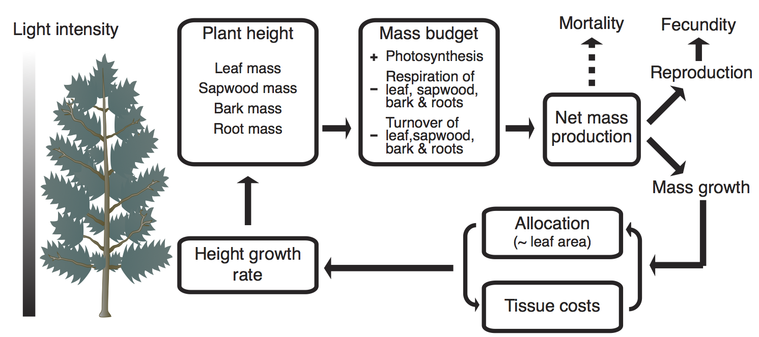
Figure 1: Physiological model in plant, giving demographic rates on the basis of its traits, size, and light environment, as functions of net mass production. The dashed arrow towards mortality indicates that, although the mortality rate is assumed to depend on mass production, no mass is actually allocated there. Figure adapted from Falster et al. (2011) and Falster, Brännström, Westoby, & Dieckmann (2015).
Growth
Leaf photosynthesis
We denote by \(p(x, E)\) the gross rate of leaf photosynthesis per unit leaf area within the canopy of a plant with traits \(x\) at light level \(E(z)\), where \(z\) is height within the canopy. We assume a relationship of the form \[\begin{equation} p(x, E(z)) = \frac{\alpha_{{\rm p1}}}{E(z) + \alpha_{{\rm p2}}}, \tag{1} \end{equation}\] for the average of \(p\) across the year. The parameters \(\alpha_{{\rm p1}}\) and \(\alpha_{{\rm p2}}\) are derived from a detailed leaf-level model and measure, respectively, maximum annual photosynthesis and the light levels at 50% of this maximum. The average rate of leaf photosynthesis across the plant is then \[\begin{equation} \bar{p}(x, H, E_{a}) = \int_0^H p(x, E_a(z)) \, q(z, H) \, {\rm d}z, \tag{2} \end{equation}\]where \(q(z, H)\) is the vertical distribution of leaf area with respect to height \(z\) (Eq. (13)).
Mass production
The amount of biomass available for growth, \({\rm d}B / {\rm d}t\), is given by the difference between income (total photosynthetic rate) and losses (respiration and turnover) within the plant (Mäkelä, 1997, Thornley & Cannell (2000), Falster et al. (2011)), \[\begin{equation} \underbrace{\strut \frac{{\rm d}B}{{\rm d}t}}_\textrm{net biomass production} = \underbrace{\strut \alpha_{\rm bio} }_\textrm{mass per C} \, \underbrace{\strut \alpha_{\rm y} }_\textrm{yield} \big( \underbrace{\strut A_{\rm l} \, \bar{p}}_\textrm{photosynthesis} - \underbrace{\strut \, \sum_{i = {\rm l}, {\rm b}, {\rm s}, {\rm r}}{M_i \, r_i}}_\textrm{respiration}\big) - \underbrace{\strut \sum_{i = {\rm l}, {\rm b}, {\rm s}, {\rm r}}{M_i \, k_i}}_\textrm{turnover}. \tag{3} \end{equation}\]Here, \(M, r\), and \(k\) refer to the mass, maintenance respiration rate, and turnover rate of different tissues, denoted by subscripts \(l\) = leaves, \(b\) = bark, \(s\) = sapwood, and \(r\) = roots. \(\bar{p}\) is the assimilation rate of CO\(_2\) per unit leaf area, \(\alpha_{\rm y}\) is yield (i.e., the fraction of assimilated carbon fixed in biomass, with the remaining fraction being lost as growth respiration; this comes in addition to the costs of maintenance respiration), and \(\alpha_{\rm bio}\) is the amount of biomass per unit carbon fixed. Gross photosynthetic production is proportional to leaf area, \(A_{\rm l} = M_{\rm l} / \phi\), where \(\phi\) is leaf mass per area. The total mass of living tissues is \(M_{\rm a} = M_{\rm l} + M_{\rm b} + M_{\rm s} + M_{\rm r}.\)
Height growth
The key measure of growth required by the demographic model is the rate of height growth, denoted \(g(x, H, E_{a})\). To model height growth requires that we translate mass production into height increment, accounting for the costs of building new tissues, allocation to reproduction, and architectural layout. Using the chain rule, height growth can be decomposed into a product of physiologically relevant terms (Falster et al., 2011), \[\begin{equation} g(x, H, E_{a}) = \frac{{\rm d}H}{{\rm d}t} = \frac{{\rm d}H}{{\rm d}A_{\rm l}} \times \frac{{\rm d}A_{\rm l} }{{\rm d}M_{\rm a}} \times \frac{{\rm d}M_{\rm a}}{{\rm d}B} \times \frac{{\rm d}B}{{\rm d}t}. \tag{4} \end{equation}\]The first factor, \({\rm d}H / {\rm d}A_{\rm l}\), is the growth in plant height per unit growth in total leaf area – accounting for the architectural strategy of the plant. Some species tend to leaf out more than grow tall, while other species emphasise vertical extension.
The second factor, \({\rm d}A_{\rm l} / {\rm d}M_{\rm a}\), accounts for the marginal cost of deploying an additional unit of leaf area, including construction of the leaf itself and various support structures. As such, \({\rm d}A_{\rm l} / {\rm d}M_{\rm a}\) can itself be expressed as a sum of construction costs per unit leaf area, \[\begin{equation} \frac{{\rm d}A_{\rm l}}{{\rm d}M_{\rm a}} = \bigg( \frac{{\rm d}M_{\rm l}}{{\rm d}A_{\rm l}} + \frac{{\rm d}M_{\rm s}}{{\rm d}A_{\rm l}} + \frac{{\rm d}M_{\rm b}}{{\rm d}A_{\rm l}} + \frac{{\rm d}M_{\rm r}}{{\rm d}A_{\rm l}}\bigg)^{-1}. \tag{5} \end{equation}\] The third factor, \({\rm d}M_{\rm a} / {\rm d}B\), is the fraction of net biomass production (Eq. (3)) that is allocated to growth rather than reproduction or storage. In theFF16 physiological model, we let this growth fraction decrease with height according to the function
\[\begin{equation}
\frac{{\rm d}M_{\rm a}}{{\rm d}B}(H) = 1 -
\frac{\alpha_{{\rm f1}}} {1 + \exp\left(\alpha_{{\rm f2}} \left(1 - H / H_{\rm mat}\right)\right)},
\tag{6}
\end{equation}\]
where \(\alpha_{{\rm f1}}\) is the maximum possible allocation (\(0-1\)) and \(\alpha_{{\rm f2}}\) determines the sharpness of the transition (Falster et al., 2011).
Diameter growth
Analogously, the growth in basal area \(A_{\rm st}\) can be expressed as the sum of growth in sapwood, bark, and heartwood areas (\(A_{\rm s}, A_{\rm b}\), and \(A_{\rm h}\), respectively), \[\begin{equation} \frac{{\rm d}A_{\rm st}}{{\rm d}t} = \frac{{\rm d}A_{\rm b}}{{\rm d}t} + \frac{{\rm d}A_{\rm s}}{{\rm d}t} + \frac{{\rm d}A_{\rm h}}{{\rm d}t}. \tag{7} \end{equation}\] Applying the chain rule, we derive an equation for basal area growth that contains many of the same elements as Eq. (4), \[\begin{equation} \frac{{\rm d}A_{\rm st}}{{\rm d}t} = \left(\frac{{\rm d}A_{\rm s}}{{\rm d}A_{\rm l}} + \frac{{\rm d}A_{\rm b}}{{\rm d}A_{\rm l}}\right) \times \frac{{\rm d}A_{\rm l}}{{\rm d}M_{\rm a}} \times \frac{{\rm d}M_{\rm a}}{{\rm d}B} \times \frac{{\rm d}B}{{\rm d}t} + \frac{{\rm d}A_{\rm h}}{{\rm d}t} . \tag{8} \end{equation}\] Diameter growth is then given by the geometric relationship between stem diameter \(D\) and \(A_{\rm st}\), \[\begin{equation} \frac{{\rm d}D}{{\rm d}t} = \left(\pi \, A_{\rm st}\right)^{-0.5} \, \frac{{\rm d}A_{\rm st}}{{\rm d}t}. \tag{9} \end{equation}\]Functional-balance model for allocation
Here we describe an allometric model linking to a plant’s height its various other size dimensions required by most ecologically realistic vegetation models (i.e., the masses of leaves, sapwood, bark, and fine roots). This approach allows us to track only the plant’s height, while still accounting for the mass needs to build leaves, roots, and stems. The growth rates of various tissues can then also be derived (Table 2).
Leaf area
Based on empirically observed allometry (Falster et al., 2011), we assume an allometric power-law scaling relationship between the accumulated leaf area of a plant and its height, \[\begin{equation} H = \alpha_{{\rm l1}} \, \left(A_{\rm l} \, {\rm m^{-2}}\right)^{\alpha_{{\rm l2}}}. \tag{10} \end{equation}\]This relationship is normalised around a leaf area of 1m\({^2}\).
Vertical distribution of leaf area
We follow the model of Yokozawa & Hara (1995) describing the vertical distribution of leaf area within the crowns of individual plants. This model can account for a variety of canopy profiles through a single parameter \(\eta\). Setting \(\eta = 1\) results in a conical canopy, as seen in many conifers, while higher values, e.g., \(\eta = 12\) , give a top-heavy canopy profile similar to those seen among angiosperms. We denote by \(A_{{\rm s},z}\) the sapwood area at height \(z\) within the plant, by \(q(z, H)\) the vertical distribution of leaf area of leaf area with respect to height \(z\), and by \(Q(z, H)\) the cumulative fraction of a plant’s leaves above height \(z\). As defined previously, \(A_{\rm s}\) is the sapwood area at the base of the plant. Following Yokozawa & Hara (1995), we assume a relationship between \(A_{{\rm s},z}\) and height such that \[\begin{equation} \frac{A_{{\rm s},z}}{A_{\rm s}} = \left(1 - \left(\frac{z}{H}\right)^\eta\right)^2. \tag{11} \end{equation}\] We also assume that each unit of leaf area is supported by a fixed area \(\theta\) of sapwood (in agreement with the pipe model; Shinozaki, Yoda, Hozumi, & Kira, 1964), so that the total canopy area of a plant relates to its basal sapwood area \(A_{\rm s}\), \[\begin{equation} A_{\rm s} = \theta \, A_{\rm l}. \tag{12} \end{equation}\]The pipe model is assumed to hold within individual plants, as well as across plants of different size. It follows that,
\[\begin{equation} Q(z, H) = \left(1-\left(\frac{z}{H}\right)^\eta\right)^2. \tag{11} \end{equation}\] Differentiating with respect to \(z\) then yields a solution for the probability density of leaf area as a function of height, \[\begin{equation} q(z, H) = 2\frac{\eta}{H}\left(1-\left(\frac{z}{H}\right)^{\eta}\right) \left(\frac{z}{H}\right)^{\eta-1}. \tag{13} \end{equation}\]Sapwood mass
Integrating \(A_{{\rm s},z}\) yields the total mass of sapwood in a plant, \[\begin{equation} M_{\rm s} = \rho \int_0^H A_{{\rm s},z} \, {\rm d}z = \rho A_{\rm s} H \eta_{\rm c} , \tag{14} \end{equation}\] where \(\eta_{\rm c} = 1 - \frac{2}{1 + \eta} + \frac{1}{1 + 2\eta}\) (Yokozawa & Hara, 1995). Substituting from Eq. (12) into Eq. (14) then gives an expression for sapwood mass as a function of leaf area and height, \[\begin{equation} M_{\rm s} = \rho \, \eta_{\rm c} \, \theta \, A_{\rm l} \, H. \tag{15} \end{equation}\]Bark mass
Bark and phloem tissue are modelled using an analogue of the pipe model, leading to a similar equation as that for sapwood mass (Eq. (15)). The cross-section area of bark per unit leaf area is assumed to be a constant fraction \(\alpha_{{\rm b1}}\) of sapwood area per unit leaf area such that \[\begin{equation} M_{\rm b} = \alpha_{{\rm b1}} M_{\rm s}. \tag{16} \end{equation}\]Root mass
Also consistent with the pipe model, we assume a fixed ratio of root mass per unit leaf area, \[\begin{equation} M_{\rm r} = \alpha_{{\rm r1}} \, A_{\rm l}. \tag{17} \end{equation}\]Even though nitrogen and water uptake are not modelled explicitly, imposing a fixed ratio of root mass to leaf area ensures that approximate costs of root production are included in calculations of carbon budget.
Seed production
The rate of seed production, \(f(x, H, E_{a})\), is a direct function of the mass allocated to reproduction, \[\begin{equation} f(x, H, E_{a}) = \frac{(1 - \frac{{\rm d}M_{\rm a}}{{\rm d}B}) \times \frac{{\rm d}B}{{\rm d}t}}{ \omega + \alpha_{{\rm f3}}}, \tag{18} \end{equation}\]where \(\omega\) is the mass of the seed and \(\alpha_{{\rm f3}}\) is the cost per seed of accessories, such as fruits, flowers, and dispersal structures. The function \(\frac{{\rm d}M_{\rm a}}{{\rm d}B}\) is the fraction of \(\frac{{\rm d}B}{{\rm d}t}\) that is allocated to growth (from Eq. (6), while \(1-\frac{{\rm d}M_{\rm a}}{{\rm d}B}\) gives the fraction allocated to reproduction).
Mortality
Instantaneous rates of plant mortality are given by the sum of a growth-independent and a growth-dependent rate (Falster et al., 2011, Moorcroft, Hurtt, & Pacala (2001)), \[\begin{equation} d(x, H, E_{a}) = d_{{\rm I}}(x, H) + d_{{\rm G}}(x, H, E_{a}). \tag{19} \end{equation}\] The growth-independent rate is taken to be constant, independent of plant performance, but potentially varying with species traits. The growth-dependent rate is assumed to decline exponentially with the rate of mass production per unit leaf area, \[\begin{equation} d_{{\rm G}}(x, H, E_{a}) = \alpha_{{\rm dG1}} \exp(-\alpha_{{\rm dG2}} X), \tag{20} \end{equation}\]where \(X = {\rm d}B/{\rm d}t / A_{\rm l}\). This relationship allows for plants to increase in mortality as their growth rate approaches zero, while allowing for species to differ in the parameters \(\alpha_{{\rm dG1}}\) and \(\alpha_{{\rm dG2}}\).
We also require a function \(S_{\rm G} (x^\prime, H_0, E_{{\rm a}0})\) for plant survival through germination. For the demographic model to behave smoothly, \(S_{\rm G} (x^\prime, H_0, E_{{\rm a}0}) / g(x, H_0, E_{{\rm a}0})\) should approach zero as \(g(x, H_0, E_{{\rm a}0})\) approaches zero. Following Falster et al. (2011), we use the function \[\begin{equation} S_{\rm G} (x^\prime, H_0, E_{{\rm a}0}) = \frac1{1 + X^2}, \tag{21} \end{equation}\]where \(X = \alpha_{{\rm d0}} \frac{A_{\rm l}}{{\rm d}B / {\rm d}t}\) and \(\alpha_{{\rm d0}}\) is a constant. Eq. (21) is consistent with Eq. (20), as both cause survival to decline with mass production.
Hyper-parameterisation of physiological model via traits
The FF16 physiological model includes default values for all needed parameters (Table 3). Species are known to vary considerably in many of these parameters, such as \(\phi\), \(\rho\), \(\nu\), and \(\omega\); so by varying parameters one can account for species differences. When altering a parameter in the model, however, one must also consider whether there are trade-offs linking parameters.
plant allows for the hyper-parameterisation of the FF16 physiological model via plant functional traits: this enables simultaneous variation in multiple parameters in accordance with an assumed trade-off. In the FF16 physiological model, we implement the relationships described below. For more details, see make_FF16_hyperpar.R.
Leaf mass per unit area
The trait leaf mass per unit area, denoted by \(\phi\), directly influences growth by changing \({\rm d}A_{\rm l} / {\rm d}M_{\rm a}\). In addition, we link \(\phi\) to the rate of leaf turnover, based on a widely observed scaling relationship from Wright et al. (2004), \[\begin{equation} k_{\rm l} = \beta_{{\rm kl1}} \, \left(\frac{\phi}{\phi_0}\right)^{-\beta_{{\rm kl2}}}. \tag{22} \end{equation}\]This relationship is normalised around \(\phi_0\), the global mean of \(\phi\). This allows us to vary \(\beta_{{\rm kl1}}\) and \(\beta_{{\rm kl2}}\) without displacing the relationship from the observed mean.
We also vary the mass-based leaf respiration rate so that it stays constant per unit leaf area and varies with \(\phi\) and nitrogen per unit leaf area \(\nu\), as empirically observed by Wright et al. (2004), \[\begin{equation} r_{\rm l} = \frac{\beta_{{\rm lf4}}\, \nu}{\phi}. \tag{23} \end{equation}\]Wood density
The trait wood density, denoted by \(\rho\), directly influences growth by changing \({\rm d}A_{\rm l} / {\rm d}M_{\rm a}\). In addition, we allow for \(\rho\) to influence the rate of growth-independent mortality, \[\begin{equation} d_{\rm I} = \beta_{{\rm dI1}} \, \left(\frac{\rho}{\rho_0}\right) ^ {-\beta_{{\rm dI2}}}, \tag{24} \end{equation}\] and also the rate of sapwood turnover, \[\begin{equation} k_{\rm s} = \beta_{{\rm ks1}} \, \left(\frac{\rho}{\rho_0}\right)^ {-\beta_{{\rm ks2}}}, \tag{25} \end{equation}\]As for \(\phi\), these relationships are normalized around \(\rho_0\), the global mean of \(\rho\). By default, \(\beta_{{\rm kI2}}\) and \(\beta_{{\rm ks2}}\) are set to zero, so these linkages only become present when these parameters are set to something other than their default values.
The rate of sapwood respiration per unit volume is assumed to be constant, so sapwood respiration per unit mass varies as \[\begin{equation} r_{\rm s} = \frac{\beta_{{\rm rs1}}}{\rho}, \tag{26} \end{equation}\] where \(\beta_{{\rm rs1}}\) is a default rate per volume of sapwood. Similarly, the rate of bark respiration per unit mass varies as \[\begin{equation} r_{\rm b} = \frac{\beta_{{\rm rb1}}}{\rho}, \tag{27} \end{equation}\]with \(\beta_{{\rm rb1}} = 2 \beta_{{\rm rs1}}\).
Seed mass
Effects of the trait seed mass, denoted by \(\omega\), are naturally embedded in the equation determining fecundity (Eq. (18)) and the initial height of seedlings. In addition, we let the accessory cost per seed be a multiple of seed size, \[\begin{equation} \alpha_{{\rm f3}} = \beta_{{\rm f1}} \omega, \tag{28} \end{equation}\]as empirically observed (Henery & Westoby, 2001).
Nitrogen per unit leaf area
Photosynthesis per unit leaf area and respiration rates per unit leaf mass (or area) are assumed to vary with leaf nitrogen per unit area, \(\nu\). The calculation of respiration rates is already described above. To calculate the average annual photosynthesis for a leaf, we integrate the instantaneous rate per unit leaf area over the annual solar trajectory, using a rectangular-hyperbolic photosynthesis light response curve, \[\begin{equation} p(\nu, E) = \frac1{365 \textrm{d}}\int_0^{365 \textrm{d}}\frac{Y(t) + A_{\rm max} - \sqrt{(Y(t) + A_{\rm max})^2 - 4 \beta_{{\rm lf2}} Y(t) A_{\rm max} }}{2 \beta_{{\rm lf2}}} {\rm d}t, \tag{29} \end{equation}\]where
- \(A_{\rm max}\) is the maximum photosynthetic capacity of the leaf,
- \(\beta_{{\rm lf2}}\) is the curvature of the light response curve,
- \(Y(t) = \beta_{{\rm lf3}} I(t)\) is the initial yield of the light response curve, with \(\beta_{{\rm lf3}}\) being the quantum yield parameter,
- \(I(t) = k_{\rm I} \, I_0(t)\, E\) is the intensity of light on the leaf surface, and
- \(I_0(t)\) is light incident on a surface perpendicular to the sun’s rays directly above the canopy at time \(t\).
The profile of \(I_0(t)\) is given by a solar model adapted from Ter Steege (1997).
We allow for the maximum photosynthetic capacity of the leaf to vary with leaf nitrogen per unit area, as \[\begin{equation} A_{\rm max} = \beta_{{\rm lf1}} \, \left(\frac{\nu}{\nu_0}\right)^{\beta_{{\rm lf5}}}, \tag{30} \end{equation}\]where \(\beta_{{\rm lf1}}\) and \(\beta_{{\rm lf5}}\) are constants. The relationships is normalized around \(\nu_0\), the global mean of leaf nitrogen per unit area.
Values of \(p(\nu, E)\) are calculated across a range of values of \(E\), and then an expression of the form in Eq. (1) is fitted to extract the parameters \(\alpha_{{\rm p1}}\) and \(\alpha_{{\rm p2}}\), such that these become functions of \(\nu\).
Tables
| Symbol | Unit | Description |
|---|---|---|
| Plant construction | ||
| \(x\) | Vector of traits for a species | |
| \(H_0\) | m | Height of a seedling after germination |
| \(H\) | m | Height of a plant |
| \(B\) | kg | Biomass originating from parent plant |
| \(M_i\) | kg | Mass of tissue type \(i\) retained on plant |
| \(A_i\) | m\(^2\) | Surface area or area of cross-section of tissue type \(i\) |
| \(q(z, H)\) | m\(^{-1}\) | Vertical distribution of leaf area across heights \(z\) for a plant with height \(H\) |
| \(Q(z, H)\) | Fraction of leaf area above height \(z\) for a plant with height \(H\)Mass production | |
| Mass production | ||
| \(p,\bar{p}\) | mol yr\(^{-1}\) m\(^{-2}\) | Photosynthetic rate per unit area |
| \(r_i\) | mol yr\(^{-1}\) kg\(^{-1}\) | Respiration rate per unit mass of tissue type \(i\) |
| \(k_i\) | yr\(^{-1}\) | Turnover rate for tissue type \(i\) |
| Environment | ||
| \(a\) | yr | Patch age |
| \(E_{a}\) | Profile of canopy openness within a patch of age \(a\) | |
| \(E_{a}(z)\) | Canopy openness at height \(z\) within a patch of age \(a\) | |
| Demographic outcomes | ||
| \(g(x, H, E_{a})\) | m yr\(^{-1}\) | Height growth rate of a plant with traits \(x\) and height \(H\) in the light environment \(E_a\) in a patch of age \(a\) |
| \(f(x, H, E_{a})\) | yr\(^{-1}\) | Seed production rate of a plant with traits \(x\) and height \(H\) in the light environment \(E_a\) in a patch of age \(a\) |
| \(d(x, H, E_{a})\) | yr\(^{-1}\) | Instantaneous mortality rate of a plant with traits \(x\) and height \(H\) in the light environment \(E_a\) in a patch of age \(a\) |
| \(S_{\rm G} (x, H_0, E_{{\rm a}0})\) | Probability that a seed germinates successfully |
| Variable | Function | Allocation | Growth.rate |
|---|---|---|---|
| (a) Assumed | |||
| Height | \(H = \alpha_{{\rm l1}} \, \left(A_{\rm l} \, {\rm m^{-2}} \right)^{\alpha_{{\rm l2}}}\) | \(\frac{{\rm d}H}{{\rm d}A_{\rm l}} = \alpha_{{\rm l2}} \alpha_{{\rm l1}} \left(A_{\rm l} \, {\rm m^{-2}} \right)^{\alpha_{{\rm l2}}-1}\) | \(\frac{{\rm d}H}{{\rm d}t} = \frac{{\rm d}H}{{\rm d}A_{\rm l}} \, \frac{{\rm d}A_{\rm l}}{{\rm d}t}\) |
| Sapwoood area | \(A_{\rm s} = \theta \, A_{\rm l}\) | \(\frac{{\rm d}A_{\rm s}}{{\rm d} A_{\rm l}} = \theta\) | \(\frac{{\rm d}A_{\rm s}}{{\rm d}t} = \frac{{\rm d}A_{\rm s}}{{\rm d} A_{\rm l}} \, \frac{{\rm d}A_{\rm l}}{{\rm d}t}\) |
| Bark area | \(A_{\rm b} = \alpha_{{\rm b1}} \, \theta \, A_{\rm l}\) | \(\frac{{\rm d}A_{\rm b}}{{\rm d} A_{\rm l}} = \alpha_{{\rm b1}} \, \theta\) | \(\frac{{\rm d}A_{\rm b}}{{\rm d}t} = \frac{{\rm d}A_{\rm b}}{{\rm d} A_{\rm l}} \, \frac{{\rm d}A_{\rm l}}{{\rm d}t}\) |
| (b) Derived | |||
| Leaf mass | \(M_{\rm l} = \phi \, A_{\rm l}\) | \(\frac{{\rm d}M_{\rm l}}{{\rm d}A_{\rm l}} = \phi\) | \(\frac{{\rm d}M_{\rm l}}{{\rm d}t} = \frac{{\rm d}M_{\rm l}}{{\rm d}A_{\rm l}} \, \frac{{\rm d}A_{\rm l}}{{\rm d}t}\) |
| Sapwood mass | \(M_{\rm s} = \rho \, \theta \, \eta_{\rm c} \, A_{\rm l} \, H\) | \(\frac{{\rm d}M_{\rm s}}{{\rm d}A_{\rm l}} = \rho \, \theta \, \eta_{\rm c} \, \big(H + A_{\rm l} \, \frac{{\rm d}H}{{\rm d}A_{\rm l}} \big)\) | \(\frac{{\rm d}M_{\rm s}}{{\rm d}t} = \frac{{\rm d}M_{\rm s}}{{\rm d}A_{\rm l}} \, \frac{{\rm d}A_{\rm l}}{{\rm d}t}\) |
| Bark mass | \(M_{\rm b} = \alpha_{{\rm b1}} \, \rho \, \theta \, \eta_{\rm c} \, A_{\rm l} \, H\) | \(\frac{{\rm d}M_{\rm b}}{{\rm d}A_{\rm l}} = \alpha_{{\rm b1}} \, \rho \, \theta \, \eta_{\rm c}\big(H + A_{\rm l} \, \frac{{\rm d}H}{{\rm d}A_{\rm l}} \big)\) | \(\frac{{\rm d}M_{\rm b}}{{\rm d}t} = \frac{{\rm d}M_{\rm b}}{{\rm d}A_{\rm l}} \, \frac{{\rm d}A_{\rm l}}{{\rm d}t}\) |
| Root mass | \(M_{\rm r} = \alpha_{{\rm r1}} \, A_{\rm l}\) | \(\frac{{\rm d}M_{\rm r}}{{\rm d}A_{\rm l}} = \alpha_{{\rm r1}}\) | \(\frac{{\rm d}M_{\rm r}}{{\rm d}t} = \frac{{\rm d}M_{\rm r}}{{\rm d}A_{\rm l}} \, \frac{{\rm d}A_{\rm l}}{{\rm d}t}\) |
| Description | Symbol | Unit | Code | Value |
|---|---|---|---|---|
| Plant construction | ||||
| Crown-shape parameter | \(\eta\) | eta | 12 | |
| Leaf mass per area | \(\phi\) | kg m\(^{-2}\) | lma | 0.1978791 |
| Wood density | \(\rho\) | kg m\(^{-3}\) | rho | 608 |
| Sapwood area per unit leaf area | \(\theta\) | theta | 0.0002141786 | |
| Height of plant with leaf area of 1m\(^2\) | \(\alpha_{\rm l1}\) | m | a_l1 | 5.44 |
| Exponent of relationship between height and leaf area | \(\alpha_{\rm l2}\) | a_l2 | 0.306 | |
| Root mass per unit leaf area | \(\alpha_{\rm r1}\) | kg m\(^{-2}\) | a_r1 | 0.07 |
| Ratio of bark area to sapwood area | \(\alpha_{\rm b1}\) | a_b1 | 0.17 | |
| Production | ||||
| Leaf photosynthesis per area | \(\alpha_{\rm p1}\) | mol yr\(^{-1}\) m\(^{-2}\) | a_p1 | 151.1778 |
| Saturation of leaf photosynthesis per area | \(\alpha_{\rm p2}\) | a_p2 | 0.2047162 | |
| Yield = fraction of carbon fixed converted into mass | \(\alpha_{\rm y}\) | a_y | 0.7 | |
| Biomass per mol carbon | \(\alpha_{\rm bio}\) | kg mol\(^{-1}\) | a_bio | 0.0245 |
| Leaf respiration per mass | \(r_{\rm l}\) | mol yr\(^{-1}\) kg\(^{-1}\) | r_l | 198.4545 |
| Fine-root respiration per mass | \(r_{\rm r}\) | mol yr\(^{-1}\) kg\(^{-1}\) | r_r | 217 |
| Sapwood respiration per mass | \(r_{\rm s}\) | mol yr\(^{-1}\) kg\(^{-1}\) | r_s | 6.598684 |
| Bark respiration per mass | \(r_{\rm b}\) | mol yr\(^{-1}\) kg\(^{-1}\) | r_b | 13.19737 |
| Turnover rate for leaves | \(k_{\rm l}\) | yr\(^{-1}\) | k_l | 0.4565855 |
| Turnover rate for sapwood | \(k_{\rm s}\) | yr\(^{-1}\) | k_s | 0.2 |
| Turnover rate for bark | \(k_{\rm b}\) | yr\(^{-1}\) | k_b | 0.2 |
| Turnover rate for fine roots | \(k_{\rm r}\) | yr\(^{-1}\) | k_r | 1 |
| Fecundity | ||||
| Seed mass | \(\omega\) | kg | omega | 0.000038 |
| Height at maturation | \(H_{{\rm mat}}\) | m | hmat | 16.59587 |
| Maximum allocation to reproduction | \(\alpha_{\rm f1}\) | a_f1 | 1 | |
| Parameter determining rate of change in\(r(x, m_\textrm{l})\) around\(H_{\rm mat}\) | \(\alpha_{\rm f2}\) | a_f2 | 50 | |
| Accessory cost per seed | \(\alpha_{\rm f3}\) | kg | a_f3 | 0.000114 |
| Mortality | ||||
| Survival probability during dispersal | \(S_{\rm D}\) | S_D | 0.25 | |
| Parameter influencing survival through germination | \(\alpha_{\rm d0}\) | kg yr\(^{-1}\) m\(^{-2}\) | a_d0 | 0.1 |
| Intrinsic or growth-independent mortality | \(d_{\rm I}\) | yr\(^{-1}\) | d_I | 0.01 |
| Baseline rate for growth-dependent mortality | \(\alpha_{\rm dG1}\) | yr\(^{-1}\) | a_dG1 | 5.5 |
| Risk coefficient for dry-mass production per unit leaf area in growth-dependent mortality | \(\alpha_{\rm dG2}\) | yr m^\({2}\) kg\(^{-1}\) | a_dG2 | 20 |
| Description | Symbol | Unit | Code | Value |
|---|---|---|---|---|
| Leaf turnover | ||||
| Global average leaf mass per area | \(\phi_0\) | kg m\(^{-2}\) | lma_0 | 0.1978791 |
| Rate of leaf turnover at average leaf mass per unit leaf area, \(\phi_0\) | \(\beta_{\rm kl1}\) | yr\(^{-1}\) | B_kl1 | 0.4565855 |
| Scaling exponent for \(\phi\) in leaf turnover | \(\beta_{\rm kl2}\) | B_kl2 | 1.71 | |
| Sapwood turnover | ||||
| Global average wood density | \(\rho_0\) | kg m\(^{-3}\) | rho_0 | 608 |
| Rate of sapwood turnover at average wood density, \(\rho_0\) | \(\beta_{\rm ks1}\) | yr\(^{-1}\) | B_ks1 | 0.2 |
| Scaling exponent for \(\rho\) in sapwood turnover | \(\beta_{\rm ks2}\) | B_ks2 | 0 | |
| Growth-independent mortality | ||||
| Rate of instantaneous mortality at average wood density, \(\rho_0\) | \(\beta_{\rm dI1}\) | yr\(^{-1}\) | B_dI1 | 0.01 |
| Scaling exponent for wood density in intrinsic mortality | \(\beta_{\rm dI2}\) | B_dI2 | 0 | |
| Photosynthesis | ||||
| Leaf nitrogen per unit leaf area | \(\nu\) | kg m\(^{-2}\) | narea | 0.00187 |
| Global average nitrogen per unit leaf area | \(\nu_0\) | kg m\(^{-2}\) | narea_0 | 0.00187 |
| Potential CO\(_2\) photosynthesis at average leaf nitrogen, \(\nu_0\) | \(\beta_{\rm lf1}\) | mol d\(^{-1}\) m\(^{-2}\) | B_lf1 | 0.8273474 |
| Curvature of light response curve | \(\beta_{\rm lf2}\) | B_lf2 | 0.5 | |
| Quantum yield of leaf photosynthesis (CO\(_2\) per unit photosynthetically active radiation) | \(\beta_{\rm lf3}\) | B_lf3 | 0.04 | |
| Scaling exponent for leaf nitrogen in maximum leaf photosynthesis | \(\beta_{\rm lf5}\) | B_lf5 | 1 | |
| Respiration | ||||
| CO\(_2\) respiration per unit leaf nitrogen | \(\beta_{\rm lf4}\) | mol yr\(^{-1}\) kg\(^{-1}\) | B_lf4 | 21000 |
| CO\(_2\) respiration per unit sapwood volume | \(\beta_{\rm rs1}\) | mol yr\(^{-1}\) m\(^{-3}\) | B_rs1 | 4012 |
| CO\(_2\)respiration per unit bark volume | \(\beta_{\rm rb1}\) | mol yr\(^{-1}\) m\(^{-3}\) | B_rb1 | 8024 |
| Reproduction | ||||
| Cost of seed accessories per unit seed mass | \(\beta_{\rm f1}\) | B_f1 | 3 |
References
Falster, D. S., Brännström, Å., Dieckmann, U., & Westoby, M. (2011). Influence of four major plant traits on average height, leaf-area cover, net primary productivity, and biomass density in single-species forests: A theoretical investigation. Journal of Ecology, 99(1), 148–164. doi:10.1111/j.1365-2745.2010.01735.x
Falster, D. S., Brännström, Westoby, M., & Dieckmann, U. (2015). Multi-trait eco-evolutionary dynamics explain niche diversity and evolved neutrality in forests. bioRxiv, 014605. doi:10.1101/014605
Henery, M., & Westoby, M. (2001). Seed mass and seed nutrient content as predictors of seed output variation between species. Oikos, 92, 479–490. doi:10.1034/j.1600-0706.2001.920309.x
Mäkelä, A. (1997). A carbon balance model of growth and self-pruning in trees based on structural relationships. Forest Science, 43, 7–24.
Moorcroft, P. R., Hurtt, G. C., & Pacala, S. W. (2001). A method for scaling vegetation dynamics: The Ecosystem Demography model (ED). Ecological Monographs, 71(4), 557–586. doi:10.1890/0012-9615(2001)071[0557:AMFSVD]2.0.CO;2
Shinozaki, K., Yoda, K., Hozumi, K., & Kira, T. (1964). A quantitative analysis of plant form - the pipe model theory. I. Basic analyses. Japanese Journal of Ecology, 14, 97–105.
Ter Steege. (1997). Winphot 5: A programme to analyze vegetation indices, light and light quality from hemispherical photographs. Georgetown, Guyana: Tropenbos Guyana Programme. Retrieved from http://www.researchgate.net/publication/230608417
Thornley, & Cannell. (2000). Modelling the components of plant respiration: Representation and realism. Annals of Botany, 85(1), 55–67. doi:10.1006/anbo.1999.0997
Wright, I. J., Reich, P. B., Westoby, M., Ackerly, D., Baruch, Z., Bongers, F., … Villar, R. (2004). The world-wide leaf economics spectrum. Nature, 428(2403), 821–827. doi:10.1038/nature02403
Yokozawa, M., & Hara, T. (1995). Foliage profile, size structure and stem diameter plant height relationship in crowded plant-populations. Annals of Botany, 76(3), 271–285.