Background

Having explored the Individual class in (Individual-level properties)[https://traitecoevo.github.io/plant/articles/individuals.html], the aim here is to use plant to investigate dynamics of many individuals within a single patch. First we instantiate the basic parameters of the FF16 strategy, particularly the probability that a patch is disturbed (via disturbance_mean_interval):

library(plant)

params <- scm_base_parameters("FF16")

params$disturbance_mean_interval <- 30.0

One patch

Next, we configure a patch containing a single species:

patch <- expand_parameters(trait_matrix(0.0825, "lma"), params, mutant = FALSE)

and run the plant characteristic solver to step the equations defining cohorts of individuals forward in time:

result <- run_scm_collect(patch)

run_scm_collect collects information about the state of the system at every ODE step:

names(result)

## [1] "time"          "species"       "env"           "seed_rain"     "patch_density" "p"

Entries are: * time: time of the step * species: a list with the state of each species (in this case there is only 1). The contents is a 3D array of variable / time step / cohort * env: a list containing 2D splines that describe the competitive environment of the patch at each step (e.g a matrix of canopy openness at a given height in the FF16 strategy) * seed_rain: the seed rain output from the patch during it’s development * p: a copy of the input parameters

First we explore patch state:

t <- result$time
h <- result$species[[1]]["height", , ]

here h is two of the three dimensions of the state array; each row is a time and each column is a cohort:

dim(h)

## [1] 142 141

While the solver ran the patch ODEs for 142 steps, the time points are not evenly distributed:

signif(t[c(1, 10, 50, 100, 142)], 1)

## [1] 0e+00 1e-04 2e-02 2e+01 1e+02

higher temporal resolution is needed to resolve early patch development, where small differences are magnified through competitive feedbacks. Our patch ran for 105 yrs, but the solver spent half the recorded steps exploring the first year alone. More on timing can be found in the cohort scheduling algorithm.

Cohorts are introduced at each time-step, except the last. At time step $i$, the rows of h record the height of all previously introduced cohorts in the patch:

h[10, 1:10]

##  [1] 0.3920954 0.3920902 0.3920850 0.3920798 0.3920746 0.3920694 0.3920642 0.3920589 0.3920537 0.3920458

with NA for cohorts that have not yet been introduced:

h[10, 11]

## [1] NA

Similarly, the $j$th column of h records the heights of a particular cohort:

h[10:19, 10]

##  [1] 0.3920458 0.3920537 0.3920617 0.3920696 0.3920776 0.3920935 0.3921094 0.3921253 0.3921412 0.3921571

with NA at time steps before it was introduced:

sum(is.na(h[, 10]))

## [1] 9

With a single species there is always one more time step than cohort introduction, with the last two steps having the same number of cohorts. With multiple species there can be more time steps than cohort introductions, as we’ll record data every cohort introduction for either species, each of which will be refined to different schedules.

In the FF16 strategy, Individuals increase in height with respect to time, but because they are competing the growth rate depends on the state of the environment (e.g. the amount of shading above an Individual’s canopy), in addition to size dependent growth.

We can plot the trajectories of cohorts developing within a patch over time:

matplot(t, h, lty=1, col=make_transparent("black", 0.25), type="l",
        las=1, xlab="Time (years)", ylab="Height (m)")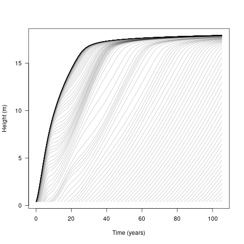

The light environment is stored over each time step, meaning that we can also plot how it changes during patch development:

# Set limits
xlim <- c(0, 1.1)
ylim <- range(result$env[[length(result$env)]][, "height"])

# Draw the spline at each step
plot(NA, xlim=xlim, ylim=ylim, las=1, xlab="Canopy openness", ylab="Height (m)")
for (i in result$env) {
  lines(i[, "canopy_openness"], i[, "height"], col="grey")
}

# Add labels at specific times
blues <- c("#DEEBF7", "#C6DBEF", "#9ECAE1", "#6BAED6",
           "#4292C6", "#2171B5", "#08519C", "#08306B")

times <- c(5, 10, 20, 40, result$time[[length(result$time)]])
cols <- colorRampPalette(blues[-(1:2)])(length(times))

for (i in seq_along(times)) {
  x <- result$env[[which.min(abs(times[[i]] - result$time))]]
  lines(x[, "canopy_openness"], x[, "height"], col=cols[[i]])

  y <- x[nrow(x), "height"]
  points(1, y, pch=19, col=cols[[i]])
  text(1 + strwidth("x"), y, paste(round(times[[i]]), "years"),
       adj=c(0, 0))
}

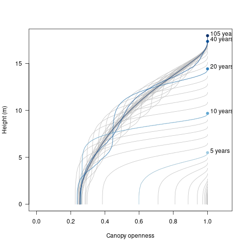initally (bottom right) all cohorts in the patch are short and the canopy is rather open (close to one). In later stages of patch development, we see that only the tallest individuals experience an open canopy. Notably, the canopy openness experienced by shorter individuals fluctuates as older individuals die and canopy gaps are filled in.

This is best shown by plotting the canopy openness at ground level over time:

y <- sapply(result$env, function(x) x[1, "canopy_openness"])
plot(result$time, y, type="l", las=1,
     ylim=c(0, 1), xlab="Time (years)", ylab="Canopy openness")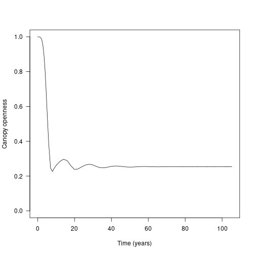

Again, the waves here are show rounds of recruitment and self thinning. Mortality is not instantaneous, so monocultures (patches of one species) recruit to a density that generates a canopy that they cannot survive under.

Multiple patches

In the FF16 strategy, leaf area index (LAI) is the driver that controls the canopy openness (via the light extinction coefficient params$k_I, following exponential extinction). This is not returned by run_scm_collect so instead we need to rebuild patches using scm_patch.

patches <- lapply(seq_along(result$time), scm_patch, result)
length(patches)

## [1] 142

Each element of the resulting list is a Patch object, the same as was observed when running the model, but at each time step. This allows us to interrogate (via the internal functions of the Patch), rather than exploring summary results. Here we calculate the competition experienced at ground level (height = 0) in terms of LAI:

lai <- sapply(patches, function(x) x$compute_competition(0.0))
plot(result$time, lai, type="l", las=1, xlab="Time (years)", ylab="Leaf area index")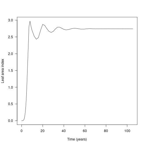

Multi-species patches

If multiple species are grown at once, they compete with one another. This adds a second species – with a higher leaf mass area (LMA) than the first species – to the population (see [Comparing Indivudals][https://traitecoevo.github.io/plant/articles/individuals.html#comparing-individuals] for a refresher on species traits)

patch_2sp <- expand_parameters(trait_matrix(0.2625, "lma"), patch, mutant = FALSE)

Then collect the patch-level dynamics:

result_2sp <- run_scm_collect(patch_2sp)

We can plot the development of each species within the patch:

t2 <- result_2sp$time
h1 <- result_2sp$species[[1]]["height", , ]
h2 <- result_2sp$species[[2]]["height", , ]

cols <- c("#e34a33", "#045a8d")

# Species 1 - red
matplot(t2, h1, lty=1, col=make_transparent(cols[[1]], .25), type="l",
        las=1, xlab="Time (years)", ylab="Height (m)")

# Species 2 - blue
matlines(t2, h2, lty=1, col=make_transparent(cols[[2]], .25))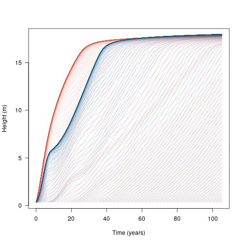

Alternatively we can compare the growth of the low LMA species (red) in a patch by itself or with another species:

# Monoculture patch (black)
matplot(t, h, lty=1, col=make_transparent("black", .25), type="l",
        las=1, xlab="Time (years)", ylab="Height (m)")

# Two species patch (red)
matlines(t2, h1, lty=1, col=make_transparent(cols[[1]], .25))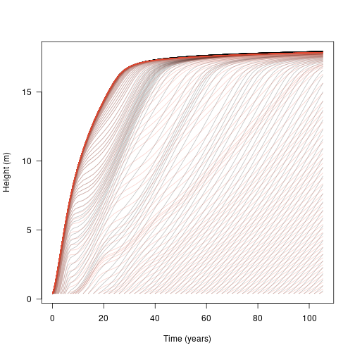

This shows that the additional species does not significantly affect the growth of the initial wave of cohorts (because the second species is growing more slowly and is shorter than the first species). However, once canopy closure has occurred (around year 5), subsequent waves of arriving cohorts are competitively suppressed, slowed or eliminated.

The dynamics are easier to see when cohort trajectories are weighted by cohort density (some of the lines here represent cohorts at close to zero density). Log density is available as a characteristic variable of all plant strategies:

# Relativise the log densities onto (-4, max)
d1 <- result_2sp$species[[1]]["log_density", , ]
d2 <- result_2sp$species[[2]]["log_density", , ]
rel <- function(x, xmin) {
  x[x < xmin] <- xmin
  xmax <- max(x, na.rm=TRUE)
  (x - xmin) / (xmax - xmin)
}
rd1 <- rel(d1, -4)
rd2 <- rel(d2, -4)

# R doesn't seem to offer a way to plot lines that vary in colour, so
# this is quite roundabout using `segments`, shaded by the density at
# the first part of the line segment:
n <- length(t2)
x <- matrix(rep(t2, ncol(h1)), nrow(h1))
col1 <- matrix(make_transparent(cols[[1]], rd1), nrow(d1))
col2 <- matrix(make_transparent(cols[[2]], rd2), nrow(d2))
plot(NA, xlim=range(t2), ylim=range(h1, na.rm=TRUE),
     las=1, xlab="Time (years)", ylab="Cohort height (m)")
segments(x[-1, ], h2[-1, ], x[-n, ], h2[-n, ], col=col2[-n, ], lend="butt")
segments(x[-1, ], h1[-1, ], x[-n, ], h1[-n, ], col=col1[-n, ], lend="butt")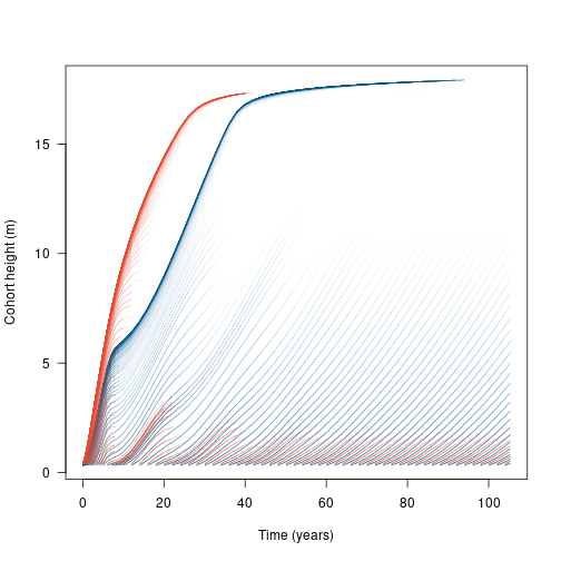

Now we see that the high LMA species (blue) becomes dominant, excluding the low LMA species (red) from the canopy.

The changing intensity of competition can be shown as the total leaf area of each species:

patches2 <- lapply(seq_along(result_2sp$time), scm_patch, result_2sp)
lai2 <- sapply(patches2, function(x) x$compute_competition(0.0))

lai2_1 <- sapply(patches2, function(x) x$species[[1]]$compute_competition(0.0))
lai2_2 <- sapply(patches2, function(x) x$species[[2]]$compute_competition(0.0))

# Patch total LAI (dashed)
plot(t2, lai2, type="l", las=1, lty=2,
     xlab="Time (years)", ylab="Leaf area index")

# Species 1 LAI (red)
lines(t2, lai2_1, col=cols[[1]])

# Species 2 LAI (blue)
lines(t2, lai2_2, col=cols[[2]])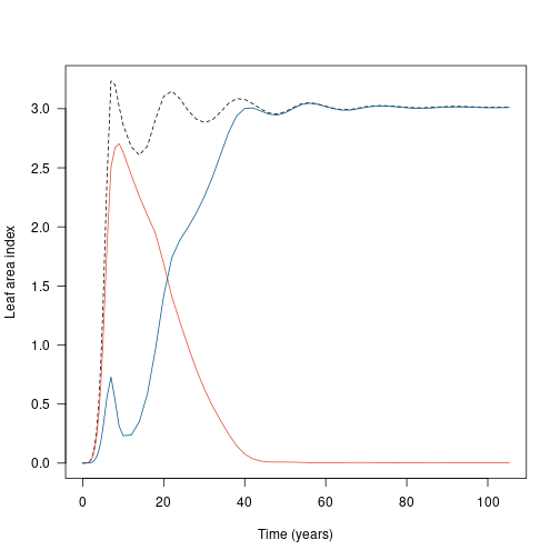

Appendix - `ggplot` example

#' A standard plot for density weighted cohort trajectories
#'
#' Parameters:
#'  - result: the output of `run_scm_collect`
#'  - threshold: lower bound on density
#' 
#' Requires:
#'  - ggplot2
#'  - dplyr

patch <- function(result, threshold = 1e-3) {

  # Unpack state and density
  t <- result$time
  h <- result$species[[1]]["height", , ]
  d <- result$species[[1]]["log_density", , ]
  n <- ncol(d)
  
  # Convert to long format
  df <- data.frame(cohort = rep(1:n, each = length(t)),
                   time = rep(t, times = n),
                   height = as.vector(h),
                   log_density = as.vector(d)) %>%
    mutate(density = exp(log_density)) 
    filter(!is.na(density))
  
  # Plot with densities
  ggplot(df, aes(x = time, y = height,
                 group = cohort, alpha = density)) +
    geom_line() + 
    labs(x = "Time (years)",
         y = "Height (m)",
         alpha = "Density") +
    theme_bw()
}

Patch-level dynamics

Rich FitzJohn

Daniel Falster

2021-02-24

Background

One patch

Multiple patches

Multi-species patches

Appendix - `ggplot` example

Patch-level dynamics

Rich FitzJohn

Daniel Falster

2021-02-24

Background

One patch

Multiple patches

Multi-species patches

Appendix - ggplot example

Appendix - `ggplot` example