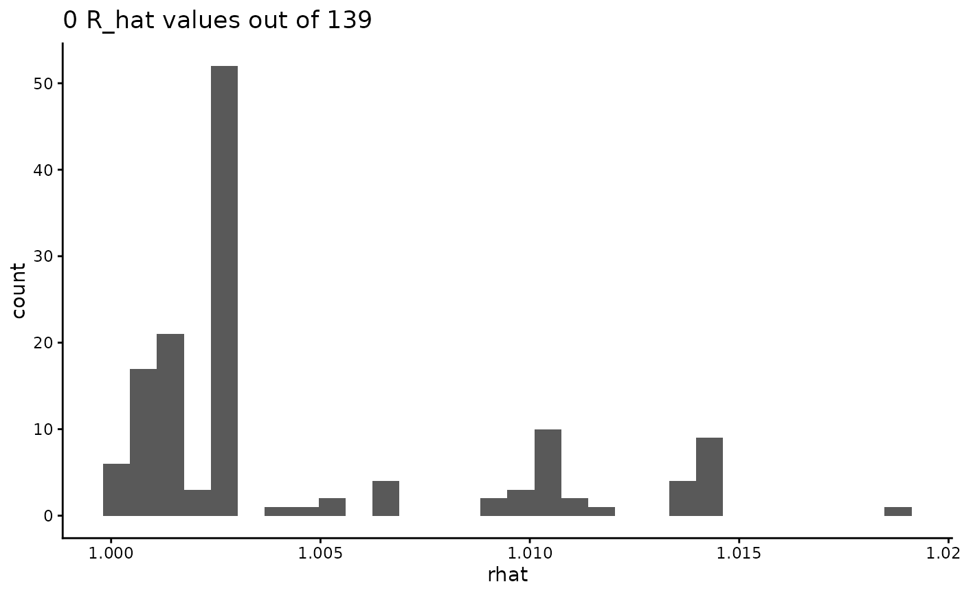
Plot histogram of R_hat values for hmde_fit object.
Source:R/hmde_plot_Rhat_hist.R
hmde_plot_Rhat_hist.RdPlot histogram of R_hat values for hmde_fit object.
Examples
# basic usage of hmde_plot_Rhat_hist
hmde_data_template("constant_single_ind",
  Trout_Size_Data[1:4,]) |>
  hmde_run(chains = 2, iter = 1000,
           verbose = FALSE, show_messages = FALSE) |>
  hmde_plot_Rhat_hist()
#>
#> SAMPLING FOR MODEL 'constant_single_ind' NOW (CHAIN 1).
#> Chain 1:
#> Chain 1: Gradient evaluation took 8e-06 seconds
#> Chain 1: 1000 transitions using 10 leapfrog steps per transition would take 0.08 seconds.
#> Chain 1: Adjust your expectations accordingly!
#> Chain 1:
#> Chain 1:
#> Chain 1: Iteration:   1 / 1000 [  0%]  (Warmup)
#> Chain 1: Iteration: 100 / 1000 [ 10%]  (Warmup)
#> Chain 1: Iteration: 200 / 1000 [ 20%]  (Warmup)
#> Chain 1: Iteration: 300 / 1000 [ 30%]  (Warmup)
#> Chain 1: Iteration: 400 / 1000 [ 40%]  (Warmup)
#> Chain 1: Iteration: 500 / 1000 [ 50%]  (Warmup)
#> Chain 1: Iteration: 501 / 1000 [ 50%]  (Sampling)
#> Chain 1: Iteration: 600 / 1000 [ 60%]  (Sampling)
#> Chain 1: Iteration: 700 / 1000 [ 70%]  (Sampling)
#> Chain 1: Iteration: 800 / 1000 [ 80%]  (Sampling)
#> Chain 1: Iteration: 900 / 1000 [ 90%]  (Sampling)
#> Chain 1: Iteration: 1000 / 1000 [100%]  (Sampling)
#> Chain 1:
#> Chain 1:  Elapsed Time: 0.01 seconds (Warm-up)
#> Chain 1:                0.007 seconds (Sampling)
#> Chain 1:                0.017 seconds (Total)
#> Chain 1:
#>
#> SAMPLING FOR MODEL 'constant_single_ind' NOW (CHAIN 2).
#> Chain 2:
#> Chain 2: Gradient evaluation took 4e-06 seconds
#> Chain 2: 1000 transitions using 10 leapfrog steps per transition would take 0.04 seconds.
#> Chain 2: Adjust your expectations accordingly!
#> Chain 2:
#> Chain 2:
#> Chain 2: Iteration:   1 / 1000 [  0%]  (Warmup)
#> Chain 2: Iteration: 100 / 1000 [ 10%]  (Warmup)
#> Chain 2: Iteration: 200 / 1000 [ 20%]  (Warmup)
#> Chain 2: Iteration: 300 / 1000 [ 30%]  (Warmup)
#> Chain 2: Iteration: 400 / 1000 [ 40%]  (Warmup)
#> Chain 2: Iteration: 500 / 1000 [ 50%]  (Warmup)
#> Chain 2: Iteration: 501 / 1000 [ 50%]  (Sampling)
#> Chain 2: Iteration: 600 / 1000 [ 60%]  (Sampling)
#> Chain 2: Iteration: 700 / 1000 [ 70%]  (Sampling)
#> Chain 2: Iteration: 800 / 1000 [ 80%]  (Sampling)
#> Chain 2: Iteration: 900 / 1000 [ 90%]  (Sampling)
#> Chain 2: Iteration: 1000 / 1000 [100%]  (Sampling)
#> Chain 2:
#> Chain 2:  Elapsed Time: 0.011 seconds (Warm-up)
#> Chain 2:                0.008 seconds (Sampling)
#> Chain 2:                0.019 seconds (Total)
#> Chain 2:
#> Warning: There were 4 divergent transitions after warmup. See
#> https://mc-stan.org/misc/warnings.html#divergent-transitions-after-warmup
#> to find out why this is a problem and how to eliminate them.
#> Warning: Examine the pairs() plot to diagnose sampling problems
#> Warning: Bulk Effective Samples Size (ESS) is too low, indicating posterior means and medians may be unreliable.
#> Running the chains for more iterations may help. See
#> https://mc-stan.org/misc/warnings.html#bulk-ess
#> Warning: Tail Effective Samples Size (ESS) is too low, indicating posterior variances and tail quantiles may be unreliable.
#> Running the chains for more iterations may help. See
#> https://mc-stan.org/misc/warnings.html#tail-ess
#> `stat_bin()` using `bins = 30`. Pick better value `binwidth`.