This vignette walks through a complete spectral-diversity workflow using only data shipped with the package, so it runs offline. The workflow has two halves that you eventually combine:
- From-the-sky: turn drone imagery into spectral-diversity metrics per area-of-interest (AOI).
- From-the-ground: turn AusPlots point-intercept data into taxonomic-diversity metrics per site.
1. Build a multiband image from single-band TIFs
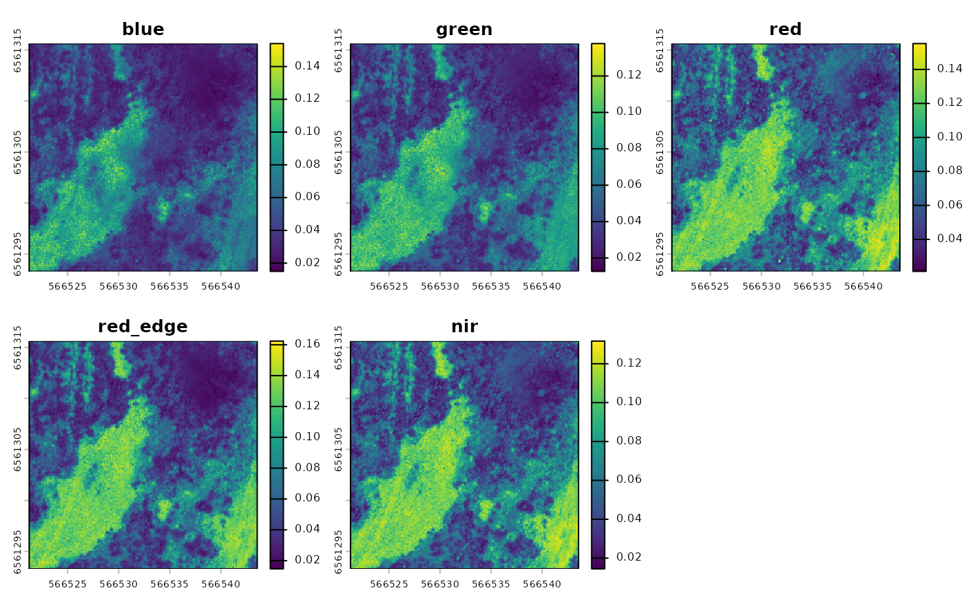
The example data ships with five single-band TIFs from a drone flight
over Fowlers Gap, NSW (blue, green,
red, red_edge, nir).
input_dir <- system.file("extdata/create_multiband_image",
                         package = "saltbush")

multiband <- create_multiband_image(
  input_dir,
  desired_band_order = c("blue", "green", "red", "red_edge", "nir"),
  output_dir = tempdir(),
  return_raster = TRUE
)
2. Choose areas of interest
We then pair the multiband image with an area-of-interest (AOI) file. The package ships a small aggregated raster and matching AOI for demonstration:
raster_files <- list.files(
  system.file("extdata/example", package = "saltbush"),
  pattern = "\\.tif$", full.names = TRUE
)

aoi_files <- list.files(
  system.file("extdata/aoi", package = "saltbush"),
  pattern = "NSABHC0009_aoi\\.shp$", full.names = TRUE
)
AOI files can be shapefiles, GeoJSON or GeoPackage. If an AOI’s coordinate system differs from the imagery’s, it is reprojected to match.
3. Calculate spectral metrics
calculate_spectral_metrics() works directly from the
rasters, cropping and masking them to each AOI, and returns three
metrics per AOI:
- CV — coefficient of variation
- SV — spectral variance
- CHV — convex hull volume
metrics <- calculate_spectral_metrics(
  raster_files, aoi_files,
  wavelengths = c("blue", "green", "red", "red_edge", "nir"),
  masked = FALSE,
  rarefaction = FALSE
)
metrics
#>         site aoi_id       CV          SV          CHV image_type
#> 1 NSABHC0009      1 0.334488 0.001761305 3.347609e-10   unmasked
4. Compute on-the-ground taxonomic diversity
For the from-the-ground side, the package ships a cached AusPlots
point-intercept dataset for the same site (NSABHC0009) so
the worked example does not need network access:
field_diversity <- calculate_field_diversity(ausplots_NSABHC0009)
field_diversity$taxonomic_diversity
#>        site_unique site_location_name species_richness shannon_diversity
#> 1 NSABHC0009-58026         NSABHC0009               52          3.056908
#> 2 NSABHC0009-53604         NSABHC0009               38          2.843074
#>   simpson_diversity pielou_evenness exp_shannon inv_simpson
#> 1         0.9203249       0.7736571    21.26171    12.55097
#> 2         0.9043699       0.7815826    17.16846    10.45696
The returned metrics are species richness, Shannon’s diversity, Simpson’s diversity, Pielou’s evenness, exponential Shannon’s, and inverse Simpson’s.
To pull a fresh query from the AusPlots database (or to query other
plots), use ausplotsR::get_ausplots():
my.data <- ausplotsR::get_ausplots(
  my.Plot_IDs = c("NSABHC0009"), veg.PI = TRUE
)
calculate_field_diversity(my.data$veg.PI)
5. Comparing the two
High-resolution drone images are very large; the example data shipped with the package is intentionally small (just enough to run examples and tests). To compare spectral and taxonomic diversity meaningfully, run the above steps on the full-resolution imagery for your own sites.
For a complete, real-world analysis built on saltbush —
including the full-resolution imagery workflow — see the companion
repository adelegem/multispectral_drone_svh.