Building your own model with external drivers

The getting-started vignette uses the Lorenz system, which ships compiled into the package. This article shows the other half of the story: how to define your own ODE system in C++ and drive it with external, time-varying forcing. It is the workflow you would follow to use odelia in your own project.

We use a simple leaf thermal model — a single ODE for leaf temperature that is forced by air temperature (an external driver) and cooled by transpiration. The complete, copy-able sources live in the installed package under system.file("examples/leaf_thermal", package = "odelia").

This is a website-only article rather than a packaged vignette, because it compiles model-specific C++ at build time. That keeps the package’s cross-platform R CMD check fast and toolchain-light.

Anatomy of an odelia model

A model that uses odelia is assembled from four files:

File	Role
src/leaf_thermal_system.hpp	The system: a C++ class defining the ODE.
src/leaf_thermal_interface.cpp	An Rcpp interface exposing the system to R.
R/leaf_thermal_interface.R	R6 wrappers giving a friendly R API.
this article	A runnable demonstration.

The system contract

A system is a class templated on its scalar type T (so the same code works with double and with the AD number type). It must implement a small contract:

template <typename T = double>
class LeafThermalSystem {
public:
  // number of state variables
  size_t ode_size() const { return ode_dimension; }

  // read state in from an iterator (and refresh drivers/rates)
  template <typename Iterator>
  Iterator set_ode_state(Iterator it, double time_);

  // write the current state out to an iterator
  template <typename Iterator>
  Iterator ode_state(Iterator it) const;

  // write the current rates (dy/dt) out to an iterator
  template <typename Iterator>
  Iterator ode_rates(Iterator it) const;
};

Templating on T is what makes the system AD-ready — see the parameter-fitting vignette.

Drivers

External forcing enters through a drivers::Drivers object. The system holds a reference to it and queries the current value on each step:

void initialize_drivers(const drivers::Drivers &drv);   // attach drivers
void set_drivers();                                     // query at current time

On the R side, Drivers fits a smooth cubic-spline interpolation through a time series, so the system can be evaluated at any time the adaptive stepper lands on. A Drivers object can hold several variables and accepts any time grid that covers the simulation.

Compile the model

Compiling a model interface requires the odelia headers on the include path. Loading odelia exposes its compiled symbols (including the XAD runtime) globally via the package .onLoad, so the temporary shared object that Rcpp::sourceCpp() builds can resolve them — no manual odelia_load_dll() call is needed.

library(odelia)

ex_dir <- system.file("examples/leaf_thermal", package = "odelia")

# Put the odelia headers on the include path for sourceCpp
Sys.setenv(PKG_CPPFLAGS = paste0("-I", system.file("include", package = "odelia")))

# Compile the model-specific interface, then load the R6 wrappers
Rcpp::sourceCpp(file.path(ex_dir, "src", "leaf_thermal_interface.cpp"), verbose = FALSE)
source(file.path(ex_dir, "R", "leaf_thermal_interface.R"))

Define drivers and run

Here the air-temperature driver is a sinusoidal daily cycle over two days.

# A daily temperature cycle
p <- list(Tmean = 32, Tamp = 6, tpeak = 15)
time_driver <- seq(0, 48, by = 0.25)
t_air <- p$Tmean + p$Tamp * sin(2 * pi * (time_driver - p$tpeak) / 24)

drivers <- Drivers$new()
drivers$set_variable("temperature", time_driver, t_air)

# Build the system with its parameters and drivers
pars <- LeafThermalSystemPars()
lz <- LeafThermalSystem$new(pars, drivers)
lz$set_state(c(25), 0) # initial leaf temperature, initial time

# Solve
ctrl <- OdeControl$new()
runner <- LeafThermalSolver$new(lz$ptr, ctrl$ptr, drivers$ptr)
times <- seq(0, 48, by = 0.5)
runner$advance_adaptive(times)

out <- runner$history()
out$time <- times
head(out)
#> # A tibble: 6 × 5
#>    time  T_LC T_air dT_LC   S_tr
#>   <dbl> <dbl> <dbl> <dbl>  <dbl>
#> 1   0    25    36.2 5.55  0.0759
#> 2   0.5  27.4  35.7 3.94  0.211 
#> 3   1    29.0  35   2.63  0.376 
#> 4   1.5  30.0  34.3 1.62  0.505 
#> 5   2    30.7  33.6 0.869 0.581 
#> 6   2.5  30.9  32.8 0.306 0.615

plot(out$time, out$T_air,
  type = "l", col = "grey50", lwd = 2,
  xlab = "time (h)", ylab = "temperature (°C)",
  ylim = range(out$T_air, out$T_LC)
)
lines(out$time, out$T_LC, col = "firebrick", lwd = 2)
legend("topright",
  legend = c("air", "leaf"),
  col = c("grey50", "firebrick"), lwd = 2, bty = "n"
)

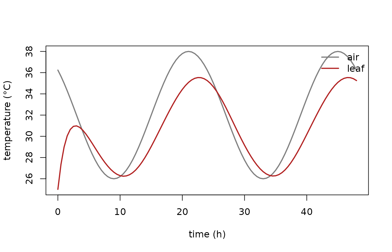
The leaf temperature tracks the air temperature but is buffered by transpirational cooling — exactly the behaviour we expect.

Comparing strategies

Because building and running a system is cheap, comparing parameterisations is just a loop. Here we double the maximum transpiration conductance and re-run:

run_strategy <- function(g_tr_max) {
  pars <- LeafThermalSystemPars()
  pars$g_tr_max <- g_tr_max
  lz <- LeafThermalSystem$new(pars, drivers)
  lz$set_state(c(25), 0)
  runner <- LeafThermalSolver$new(lz$ptr, ctrl$ptr, drivers$ptr)
  runner$advance_adaptive(times)
  runner$history()$T_LC
}

base_g <- LeafThermalSystemPars()$g_tr_max
T_baseline <- run_strategy(base_g)
T_high_cond <- run_strategy(2 * base_g)

plot(times, out$T_air,
  type = "l", col = "grey70", lwd = 2,
  xlab = "time (h)", ylab = "leaf temperature (°C)",
  ylim = range(out$T_air, T_baseline, T_high_cond)
)
lines(times, T_baseline, col = "firebrick", lwd = 2)
lines(times, T_high_cond, col = "steelblue", lwd = 2)
legend("topright",
  legend = c("air", "baseline", "2x conductance"),
  col = c("grey70", "firebrick", "steelblue"), lwd = 2, bty = "n"
)

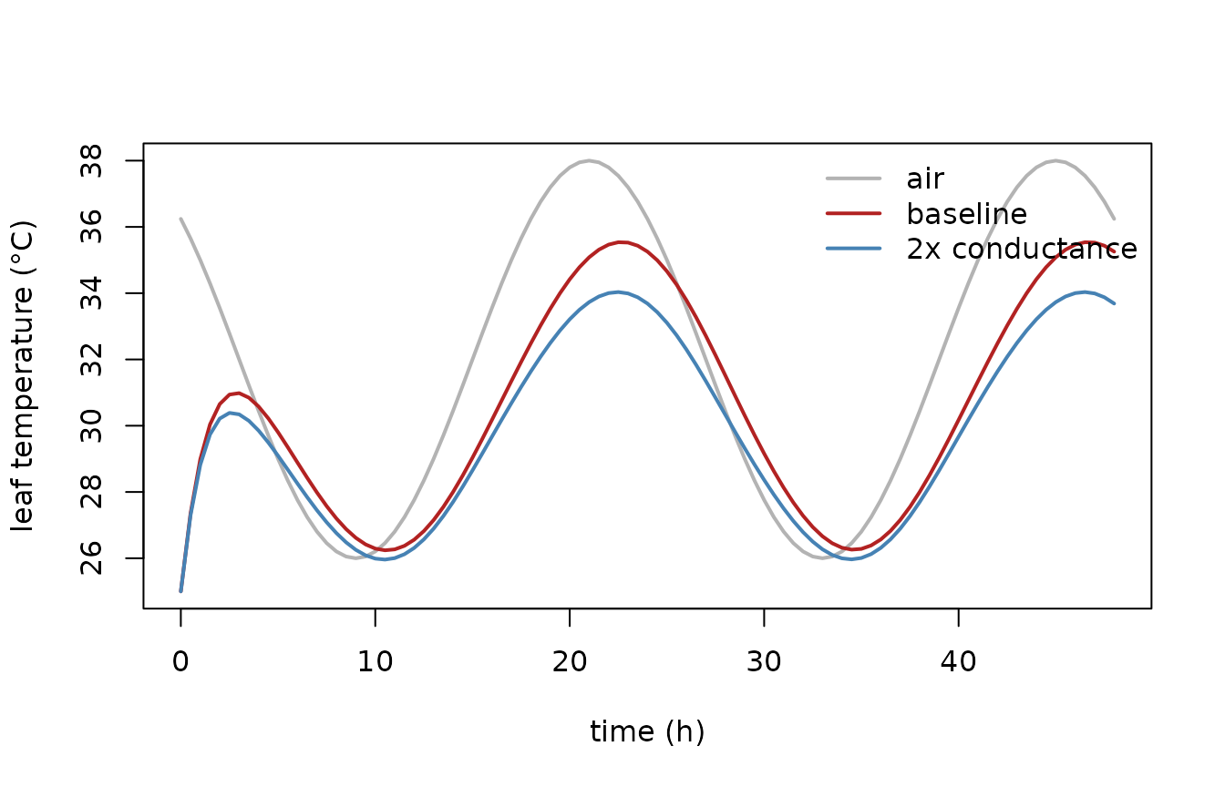
Higher conductance means stronger transpirational cooling, so the leaf stays closer to — or below — air temperature at the hottest part of the day.

Where next

• The full, copy-able sources are in system.file("examples/leaf_thermal", package = "odelia") — start there when building your own model.
• To calibrate a model’s parameters against data using exact gradients, see the parameter-fitting vignette.