library(dplyr)
library(tidyr)
library(ggplot2)
library(purrr)
library(deSolve)Prototyping a soil water-balance bucket model
experimental
soil-water
An early deSolve prototype exploring soil water dynamics — infiltration, drainage, diffusivity flux, and Penman-Monteith evaporation.
Note
This is an exploratory experiment from 2021, kept for the record. It prototypes soil water dynamics directly with deSolve and does not use the plant package API — it is not maintained and may not reflect the current model.
Originally authored by Isaac Towers, 2021-05-19.
Here I will develop the prototype for the water bucket model for the plant model tracking the rate of change in \(\theta\)
\[\frac{d\theta}{dt} = \frac{1}{z}\bigg({R\,I(\theta) - E_T (\theta) - E_S (\theta) - J(\theta)}\bigg) \]
Variables
\(\theta ( t)\): soil volumetric water content \((m^3 / m^3)\)
Parameters
\(R\): Rainfall \((m^3 m^{-2} / t)\) \(I\): Infiltration rate (unitless) \(E_T\): Transpiration (water used by plants) \((m^3 m^{-2} / t)\) \(E_S\): Soil surface evaporation \((m^3 m^{-2} / t)\) \(J\): Drainage from soil profile \((m^3 m^{-2} /t)\) \(z\): Soil depth (m)
\[I(\theta) = 1-\bigg(\frac{\theta(t)}{\theta_{sat}}\bigg)^b\]
\(b\): Unitless parameter determining the shape of water accumulation in the soil moisture bank \(\theta_{sat}\) Soil moisture capacity \((m^3 m^{-3})\)
Ok, lets first show that rain will eventually fill up the soil without any water outputs if we include a saturated water content
\[\frac{d\theta}{dt} = R *\bigg(1-\bigg(\frac{\theta(t)}{\theta_{sat}}\bigg)^b\bigg)\]
# Timestep
t <- seq(0,365, by = 1)

# Variables
theta_init <- c(theta=0.210)

# Model parameters
params <-
  expand_grid(theta_sat = 0.513,
            R  = 1000/365,
            b = c(1, 0.5, 2, 4, 8),
            z = 1000) %>%
        split(., .$b)

# Rates of change
theta_rates <- function(t, theta, params) {
  with(as.list(c(theta, params)), {

    dtheta_dt = (R*(1-(theta/theta_sat)^b))/z

    return(list(c(dtheta_dt)))
  })
}
logistic_solution <-
map_dfr(
params,
~ode(
y = theta_init,
times = t,
func = theta_rates,
parms = .x) %>%
as.data.frame(), .id = "b")logistic_solution %>%
ggplot(aes(time, theta, col=b)) +
geom_line()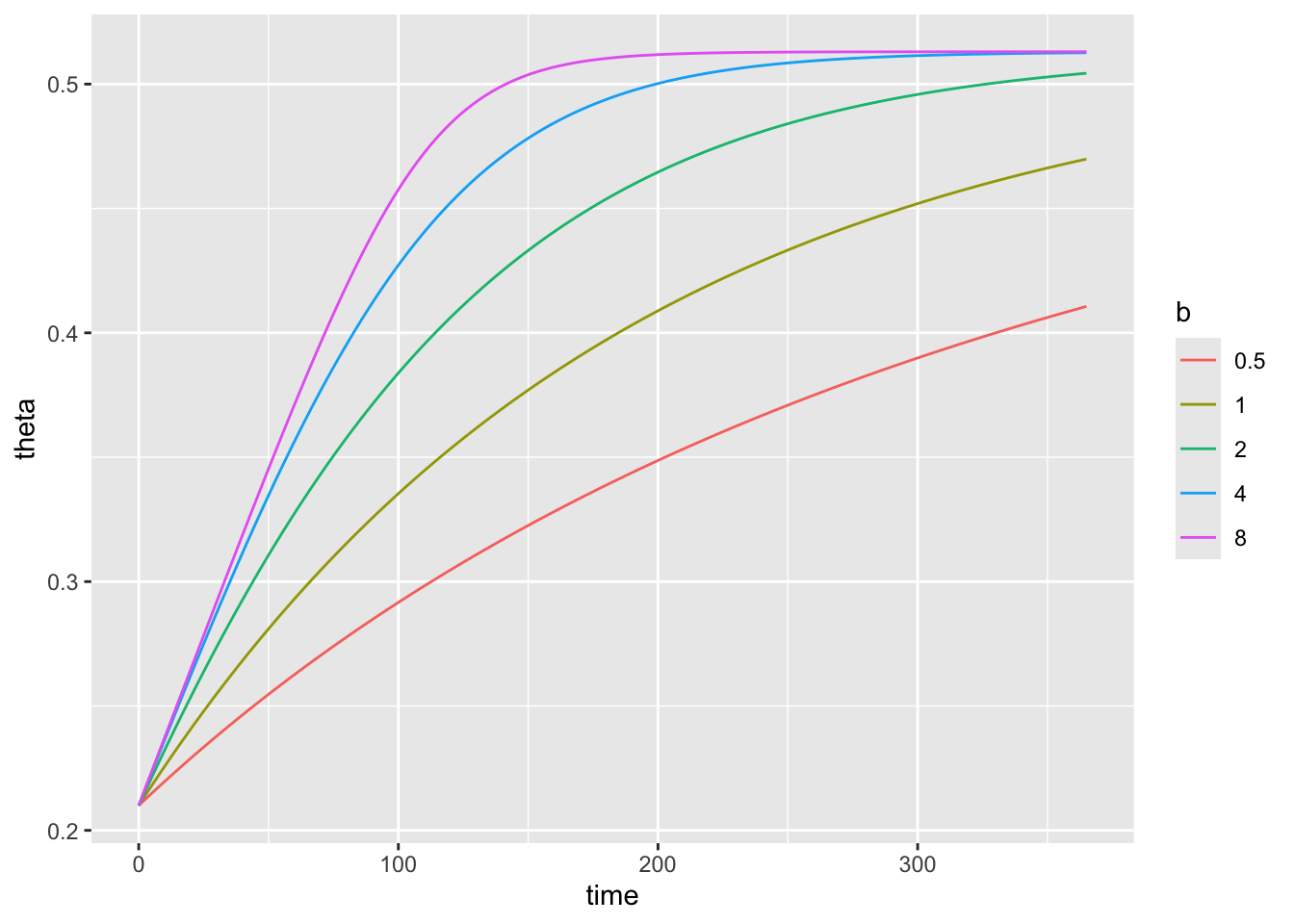
Cool, let’s now include a drainage factor.
The soil moisture content in the top layer of soil is defined the soil moisture between 0m depth and the first monited depth point as follows:
\[\frac{d\theta_1}{dt} = \frac{1}{z_1}\bigg(R\,I-J_1\bigg),\]
where rainfall enters the soil and drains at rate: \(J\) and \(1\) represents the first monitored soil depth.
For all layers below the first, the soil moisture content is defined as follows:
\[\frac{d\theta_i}{dt} = \frac{1}{z_i - z_{i-1}}\bigg(J_{i-1}-J_i\bigg)~i>1,\]
where \(J_{i-1}\) is the drainage of soil water from above.
Because we are still unsure about how water flux works with regards to the balance bewteen matric and gravitational potential, we will use a much more simplified version of water flux employed by Duursma and Medlyn (2012) where water is assumed to only travel downwards and is directly equivalent to the soil hydraulic conductivity \(K_z~( m~day^{-1})\)):
\[J_i= -K_z(\theta),\]
where:
\[K_z= K_{sat}(\frac{\theta}{\theta_{sat}})^{nk},\]
and \(K_{sat}\) \((m~day^{-1})\) and \(nk\) (unitless) are empirical parameter which vary with soil type
# Timestep
t <- seq(0,365, by = 1)

# Variables
theta_init <- c(theta1=0.513, theta2=0, theta3=0)

# Model parameters for silty loam (Landsberg)
params <-
  expand_grid(theta_sat = 0.513,
    R  = 1/365,
    #convert to day
    ksat = c(12.2*24),
    nk = 11.9
    ) %>%
        split(., .$ksat)

# Rates of change
theta_rates <- function(t, theta, params) {
  with(as.list(c(theta, params)), {
    dtheta1_dt = R - (ksat * (theta1/theta_sat)^nk)/0.1
    dtheta2_dt = ((ksat * (theta1/theta_sat)^nk) - (ksat * (theta2/theta_sat)^nk))/0.5
    dtheta3_dt = ((ksat * (theta2/theta_sat)^nk))/0.5
    return(list(c(dtheta1_dt,dtheta2_dt,dtheta3_dt)))
  })
}
logistic_solution <-
map_dfr(
params,
~ode(
y = theta_init,
times = t,
func = theta_rates,
parms = .x) %>%
as.data.frame(), .id = "ks")logistic_solution %>%
ggplot(aes(time)) +
geom_line(aes(y = theta1, col="Top Layer")) +
geom_line(aes(y = theta2, col="Middle Layer")) +
geom_line(aes(y = theta3, col="Bottom Layer"))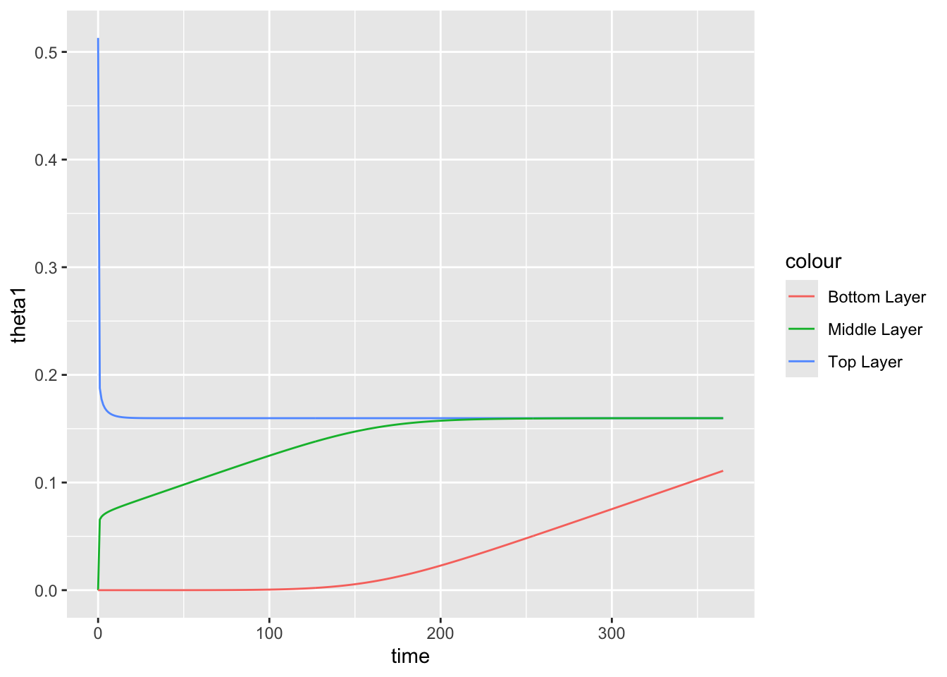
An alternative which does allow for upwards flux is to calculate water flux based on diffusivity,D, \((m^2~yr^{-1})\):
\[J_i = -D_s\frac{\delta\theta_s}{\delta z},\]
where D is equal to:
\[D(\theta) = D_{sat}(\frac{\theta_s}{\theta_{sat}})^{n_D}.\]
In this example, \(\delta z\) is calculated as:
\[\delta z = z_{i+1} - z_i,\]
and the same for \(\delta \theta\):
\[\delta \theta = \theta_{s,i+1} - \theta_{s,i}.\]
# Timestep
t <- seq(0,1000, by = 0.1)

# Variables
theta_init <- c(theta11=0, theta22=0, theta33=0, theta44=0)


# Model parameters for silty loam (Landsberg)
params <- list(
  c(
    R=3/365,
    dsat = 1.4,
    nd = 6.5,
    theta_sat = c(0.482),
    b=8,
    amp=0,
    I_constant=1,
    sine_height=1,
    frequency=180,
    ksat=292.8,
    nk=11.9
    ))


# Rates of change
theta_rates1 <- function(t, theta_init, params) {
  with(as.list(c(theta_init, params)), {
    dtheta1_dt=R-(-dsat*(theta11/theta_sat)^nd)*((theta22-theta11)/0.50)
    dtheta2_dt=(-dsat*(theta11/theta_sat)^nd)*((theta22-theta11)/0.50)-(-dsat*(theta22/theta_sat)^nd)*((theta33-theta22)/0.50)
    dtheta3_dt=(-dsat*(theta22/theta_sat)^nd)*((theta33-theta22)/0.50)-((ksat)*(theta33/theta_sat)^nk)
    dtheta4_dt=((ksat)*(theta33/theta_sat)^nk)

    return(list(c(dtheta1_dt,dtheta2_dt,dtheta3_dt,dtheta4_dt)))
  })
}
logistic_solution1 <-
map_dfr(
params,
~ode(
y = theta_init,
times = t,
func = theta_rates1,
parms = .x) %>%
as.data.frame())The same idea, now wired up as a general multi-layer model with configurable monitored depths, runoff and deep-drainage bookkeeping, and a seasonal rainfall signal.
#set time period and time step
t <- seq(0,1000, by = 1)

#how many soil depths should be monitored
n=3

#set depth of points, can be customised. N-1 in this case accounts for one customsied point, all others are the same
standard_depth = 0.5
z <- c(0.10, rep(standard_depth, n-1))

i=1

#set vector to collect gradients
dtheta_dt <- vector(length = n)

#set initial soil moisture content for each layer (boundary z[i] - z[i-1]) as well as the amount of water lost to deep drainage and runoff and the total amount of rainfall falling in period for sanity check, particulary important for when inclduing temporal variation
theta_init <- c(theta=rep(0, n), runoff = 0, deep_drainage=0, cumulative_rain=0)

#set parameter values
params <- list(
  c(
    R=3/365,
    dsat = 1.4,
    nd = 6.5,
    theta_sat = 0.482,
    b=8,
    ksat=292.8,
    nk=11.9,
    amp=1,
    sine_height=1,
    frequency=180,
    I_constant = 1
    ))
#soil moisture drainage model

theta_rates <- function(t, theta, params) {
  with(as.list(c(theta, params)), {

    I = (1-I_constant*(theta[i]/theta_sat)^b)
    S = amp*sin(t/frequency*pi)+sine_height

    for(i in 1:n){

    #top layer. Non-infiltrating rainfall is stored in runoff, but leaves the plant-accessible water budget forever.
      if(i == 1) {
    inflow = R*S*I
    runoff = (R*S)*(1-I)
    outflow = (-dsat*(theta[i]/theta_sat)^nd)*((theta[i+1]-theta[i])/z[i+1])

      }

    #middle layers
      if(!i %in% c(1, n)) {
     inflow = (-dsat*(theta[i-1]/theta_sat)^nd)*((theta[i]-theta[i-1])/z[i])
     outflow= (-dsat*(theta[i]/theta_sat)^nd)*((theta[i+1]-theta[i])/z[i+1])
      }

    # last layer - water that outflows from this layer is gone forever. Values are stored in deep_drainage.
      if(i == (n)) {
    inflow = (-dsat*(theta[i-1]/theta_sat)^nd)*((theta[i]-theta[i-1])/z[i])
    outflow = ((ksat)*(theta[i]/theta_sat)^nk)
    deep_drainage = ((ksat)*(theta[i]/theta_sat)^nk)
      }

    dtheta_dt[i] = inflow - outflow
    runoff = runoff
    deep_drainage = deep_drainage
    cumulative_rain = R*S
    }

    return(list(c(dtheta_dt, runoff, deep_drainage, cumulative_rain)))
  })
}
logistic_solution <-
map_dfr(
params,
~ode(
y = theta_init,
times = t,
func = theta_rates,
parms = .x) %>%
as.data.frame())logistic_solution %>%
select(time, contains("theta")) %>%
pivot_longer(., contains("theta")) %>%
rename(Soil_depth = name) %>%
ggplot(aes(time)) +
geom_line(aes(y=value, col=Soil_depth))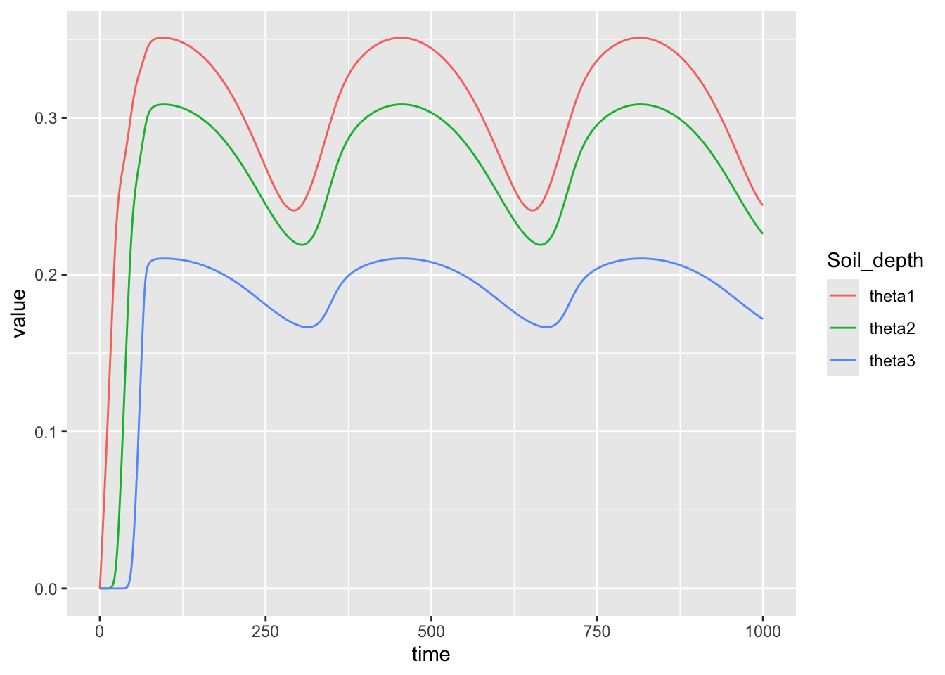
A hard-coded ten-layer expansion of the same scheme, kept here as scratch working.
#ignore below for now


# Timestep
t <- seq(0,1000, by = 0.1)

# Variables
theta_init <- c(theta1=0, theta2=0, theta3=0, theta4=0, theta5=0, theta6=0, theta7=0, theta8=0, theta9=0, theta10=0, runoff = 0)


# Model parameters for silty loam (Landsberg)
params <- list(
  c(
    R=3/365,
    dsat = 1.4,
    nd = 6.5,
    theta_sat = c(0.482),
    b=8,
    I_constant=1,
    amp=0,
    sine_height=1,
    frequency=180,
    ksat=292.8,
    nk=11.9))

# Rates of change
theta_rates <- function(t, theta_init, params) {
  with(as.list(c(theta_init, params)), {
    I = (1-(theta1/theta_sat)^b)
    S = amp*sin(t/frequency*pi)+sine_height
    dtheta1_dt=R*S*I-(-dsat*(theta1/theta_sat)^nd)*((theta2-theta1)/0.25)
    dtheta2_dt=((-dsat*(theta1/theta_sat)^nd)*((theta2-theta1)/0.25)-(-dsat*(theta2/theta_sat)^nd)*((theta3-theta2)/0.25))
    dtheta3_dt=((-dsat*(theta2/theta_sat)^nd)*((theta3-theta2)/0.25)-(-dsat*(theta3/theta_sat)^nd)*((theta4-theta3)/0.25))
    dtheta4_dt=((-dsat*(theta3/theta_sat)^nd)*((theta4-theta3)/0.25)-(-dsat*(theta4/theta_sat)^nd)*((theta5-theta4)/0.25))
    dtheta5_dt=((-dsat*(theta4/theta_sat)^nd)*((theta5-theta4)/0.25)-(-dsat*(theta5/theta_sat)^nd)*((theta6-theta5)/0.25))
    dtheta6_dt=((-dsat*(theta5/theta_sat)^nd)*((theta6-theta5)/0.25)-(-dsat*(theta6/theta_sat)^nd)*((theta7-theta6)/0.25))
    dtheta7_dt=((-dsat*(theta6/theta_sat)^nd)*((theta7-theta6)/0.25)-(-dsat*(theta7/theta_sat)^nd)*((theta8-theta7)/0.25))
    dtheta8_dt=((-dsat*(theta7/theta_sat)^nd)*((theta8-theta7)/0.25)-(-dsat*(theta8/theta_sat)^nd)*((theta9-theta8)/0.25))
    dtheta9_dt=((-dsat*(theta8/theta_sat)^nd)*((theta9-theta8)/0.25))-((ksat)*(theta9/theta_sat)^nk)
    dtheta10_dt= ((ksat)*(theta9/theta_sat)^nk)
    # ((12.2*24)*(theta9/theta_sat)^11.9)
    runoff = R*S*(1-I)

    return(list(c(dtheta1_dt,dtheta2_dt, dtheta3_dt,dtheta4_dt,dtheta5_dt,dtheta6_dt,dtheta7_dt,dtheta8_dt,dtheta9_dt,dtheta10_dt
, runoff)))
  })
}
logistic_solution <-
map_dfr(
params,
~ode(
y = theta_init,
times = t,
func = theta_rates,
parms = .x) %>%
as.data.frame())logistic_solution %>%
ggplot(aes(time)) +
geom_line(aes(y = theta1, col="1st Layer")) +
geom_line(aes(y = theta2, col="2nd Layer")) +
geom_line(aes(y = theta3, col="3rd Layer"))+
geom_line(aes(y = theta4, col="4th Layer"))+
geom_line(aes(y = theta5, col="5th Layer"))+
geom_line(aes(y = theta6, col="6th Layer"))+
geom_line(aes(y = theta7, col="7th Layer"))+
geom_line(aes(y = theta8, col="8th Layer"))+
geom_line(aes(y = theta9, col="9th Layer"))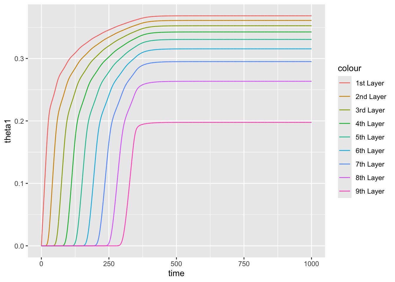
Now let’s add evaporation. We will use the Penman-Monteith equation to model evaporation as a water flux (rather than an energy flux):
\[E=\frac{\Delta*\varphi_s+g_a*p_a*c_{pa}*D}{\Delta+\gamma(1+\frac{g_a}{g_s})}*\frac{1}{L},\]
Where E is the evaporation in m (i.e. \(mm\)). This equation is dependent on the air temperature, which manifests its effect on evaporation through determining the vapour pressure deficit \(D\), and the derivative of the saturated vapour pressure curve at a given air temperature \(\Delta\), the net radiation reaching the soil surface \(\varphi_s\), and soil moisture which affects the soil conductance \(g_s\).
The equation for the saturated vapour pressure is dependent on air temperature \((T_{air}~(^\circ C))\) only:
\[e_s=0.6108\exp\bigg(\frac{17.27*T_{\rm air}}{T_{\rm air} + 237.3}\bigg).\]
Thus, \[\Delta = \frac{\delta e_s}{\delta T_{air}}.\]
To estimate the daily average vapour pressure deficit, the maximum \(T_{max}\) and minimum \(T_{min}\) air temperature can be used \[\overline{D} = e_s(T_{\rm max})-e_s(T_{\rm min}),\]
and the daytime average vapour pressure deficit \(D_sd\) can be calculated by assuming a fraction of daytime hours \(\alpha\): \[\overline{D_{daytime}} = \alpha * e_s(T_{max})- (1-\alpha) * e_s(T_{min}).\]
Radiation reaching the soil surface (i.e. passing through the tree canopy) is assumed to be entirely absorbed. Thus, net radiation at the soil surface is defined as the radiation incident on the tree canopy \(\varphi_0\) minus the radiation absorbed the tree canopy \(\varphi_na\)
\[\varphi_s = \varphi_0 - \varphi_{na},\]
where \(\varphi_{na}\) is dependent on the leaf area index (LAI) of the canopy and the light extinction coefficient (k):
\[\varphi_{na} = \varphi_0*(1-e^{-k*LAI})\]
Conductance of water vapour through the soil moisture boundary layer \(g_c\) is dependent on soil moisture, because resistance to evaporation increases as the soil becomes increasingly dry according the following equation. Using an equation proposed by Soares and Almeida (2001):
\[g_{s} = g_{s_{max}}*(\theta/\theta_{sat})\]
Once through the soil moisture boundary layer, water vapour must then travel through the atmospheric boundary layer according to the rate \(g_a\). For soil, a fixed value is currently assumed using value obtained from Soares and Almeida (2001) where \(g_{a_s} = 0.01 m~s^{-1}\)
# Timestep
t <- seq(0,3650, by = 1)

# Variables
theta_init <- c(theta=0.513)

# Model parameters
params <-
  expand_grid(theta_sat = 0.513,
            R  = 1000/365,
            b = 8,
            gcmax=0.0025,
            gb=0.01,
            vpd=900,
            p = 1.204,
            cpa = 1004,
            y=66.1,
            s=145,
            air_temp=25,
            slope_sat_vap_curve = 4098*(0.6108*exp((17.27*air_temp)/(air_temp+237.3)))/(air_temp+237.3)^2 *1000,
            #radiation will be fed in from plant model based on its solar radiation submodel and plant lai
            rad = c(200,434),
            max_air_temp = 25,
            min_air_temp= 10,
            L = 2.45*10^6,
            z = 1500) %>%
            split(., .$rad)

# Rates of change
theta_rates <- function(t, theta, params) {
  with(as.list(c(theta, params)), {
    evap_numerator = slope_sat_vap_curve *rad + gb*p*cpa*vpd
    evap_denominator = slope_sat_vap_curve + y*(1+gb/(gcmax*(theta/theta_sat)))
    evap=evap_numerator/evap_denominator*(1/L)*12*60*60
    dtheta_dt = (R*(1-(theta/theta_sat)^b)- evap)/z

    return(list(c(dtheta_dt)))
  })
}
logistic_solution <-
map_dfr(
params,
~ode(
y = theta_init,
times = t,
func = theta_rates,
parms = .x) %>%
as.data.frame(), .id = "rad")logistic_solution %>%
ggplot(aes(time, theta, col=rad)) +
geom_line()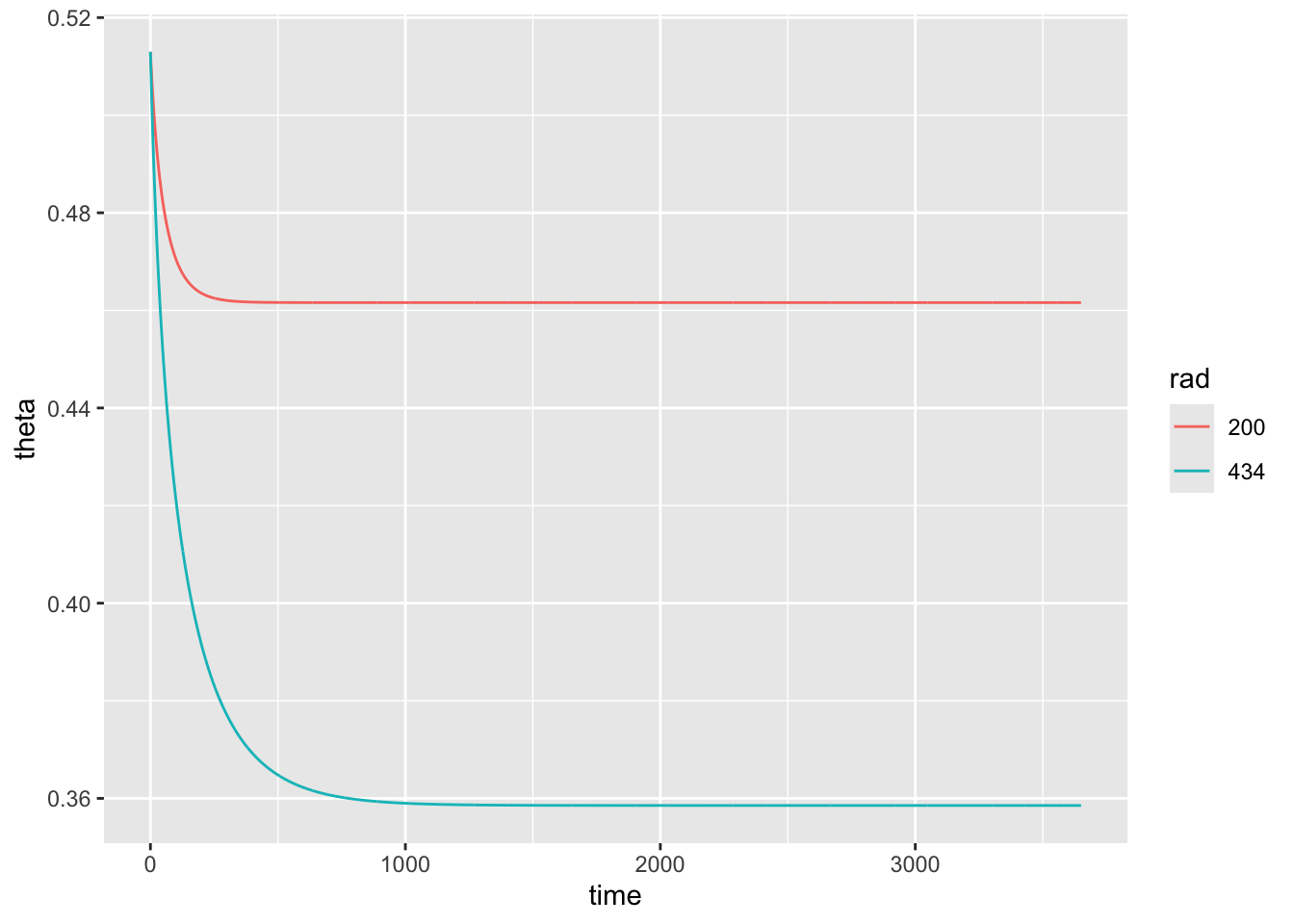
# Timestep
t <- seq(0,100, by = 0.1)

# Variables
theta_init <- c(theta1=0.513, theta2=0, theta3=0)

# Model parameters
params <-
  expand_grid(
    theta_sat = 0.513,
    ds = 0.86,
    nd = 8.5,
    R = 0.00274
    ) %>%
        split(., .$ds)

# Rates of change
theta_rates <- function(t, theta, params) {
  with(as.list(c(theta, params)), {

    dtheta_dt1 = R -(ds*((theta1/theta_sat)^nd)) * (theta1-theta2)
    dtheta_dt2 = ((ds*((theta1/theta_sat)^nd)) * (theta1-theta2)) - ((ds*((theta2/theta_sat)^nd)) * (theta2-theta3))
    dtheta_dt3 = ((ds*((theta2/theta_sat)^nd)) * (theta2-theta3))

    return(list(c(dtheta_dt1,dtheta_dt2,dtheta_dt3)))
  })
}
logistic_solution <-
map_dfr(
params,
~ode(
y = theta_init,
times = t,
func = theta_rates,
parms = .x) %>%
as.data.frame(), .id = "ks")logistic_solution %>%
ggplot(aes(time, theta1, col=ks)) +
geom_line()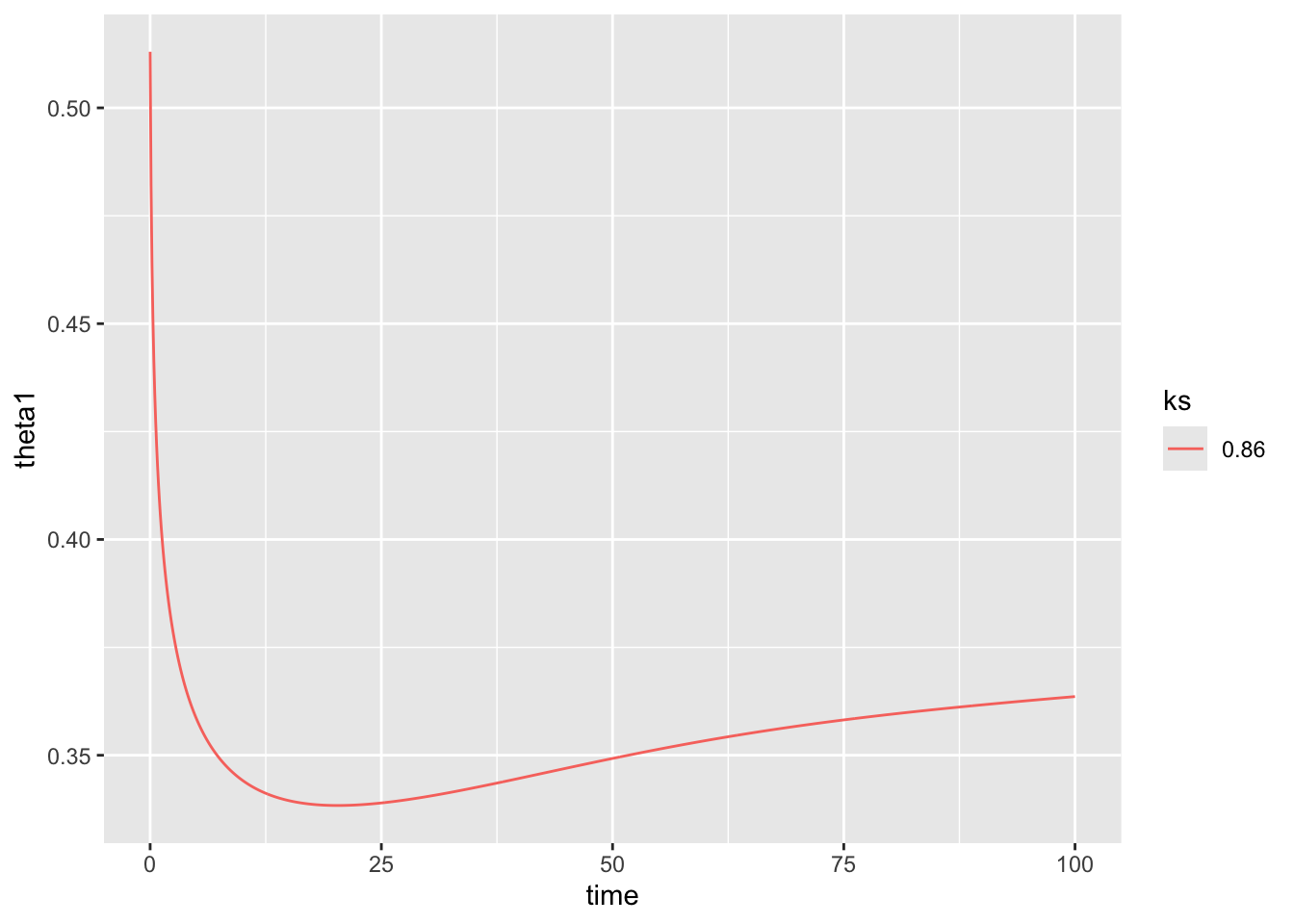
logistic_solution %>%
  ggplot(aes(time, theta2, col=ks)) +
  geom_line()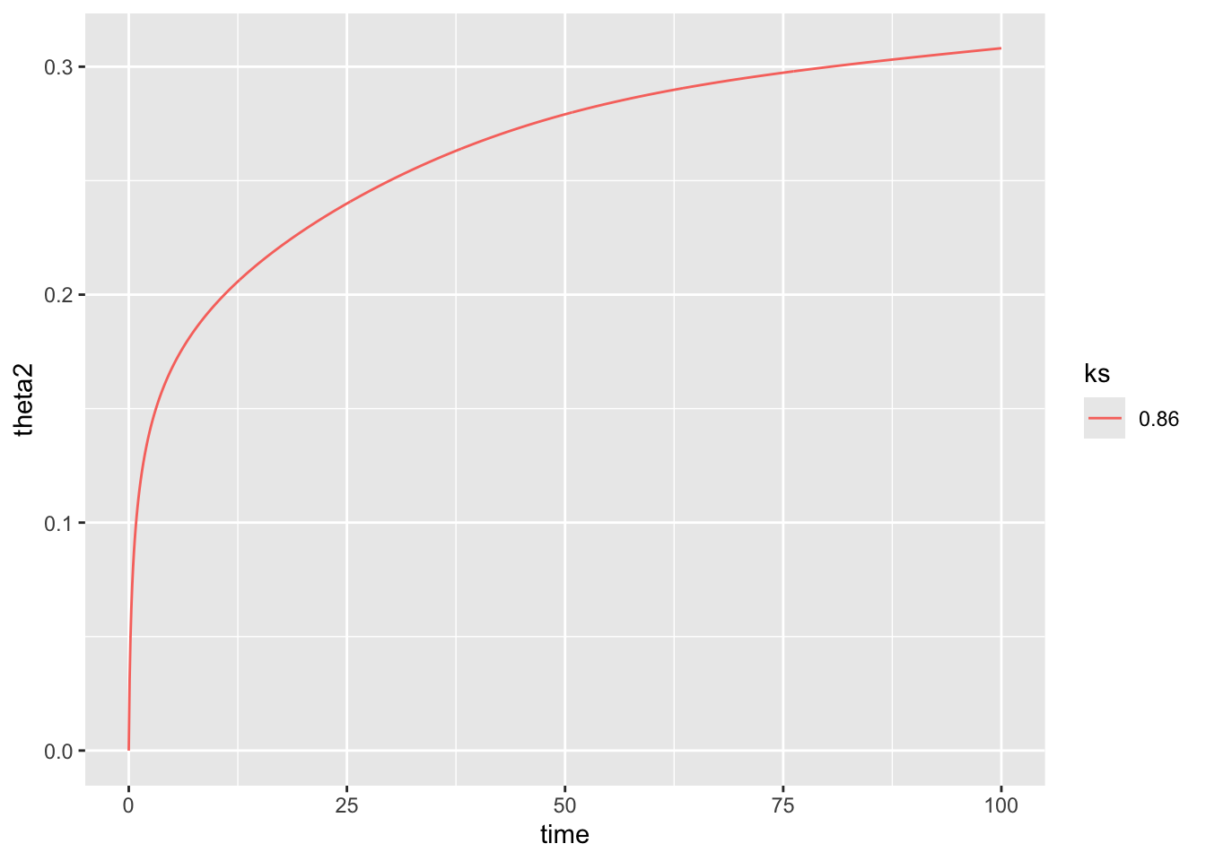
logistic_solution %>%
  ggplot(aes(time, theta3, col=ks)) +
  geom_line()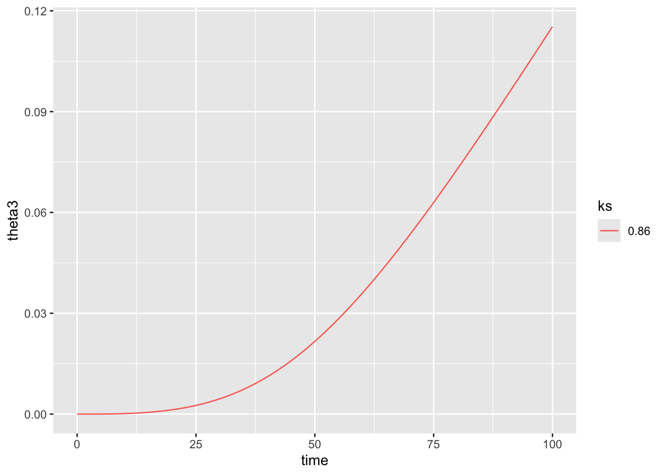
# Timestep
t <- seq(0,10, by = 0.1)

# Variables
theta_init <- c(theta=0.482)

# Model parameters
params <-
  expand_grid(
    ks = c(0.00021388),
    theta_sat = 0.482,
    nk = 0.007,
    g = 9.8,
    pw = 1000,
    apsi = 1.87,
    npsi = 11.3) %>%
        split(., .$ks)

# Rates of change
theta_rates <- function(t, theta, params) {
  with(as.list(c(theta, params)), {

    dtheta_dt = -(((ks*(theta/theta_sat)^nk)/(g*pw)) * apsi * npsi * theta^(-npsi-1))

    return(list(c(dtheta_dt)))
  })
}
logistic_solution <-
map_dfr(
params,
~ode(
y = theta_init,
times = t,
func = theta_rates,
parms = .x) %>%
as.data.frame(), .id = "ks")DLSODA- Warning..Internal T (=R1) and H (=R2) are
such that in the machine, T + H = T on the next step
(H = step size). Solver will continue anyway.
In above message, R1 = 9.93182, R2 = 8.29801e-16
DLSODA- Warning..Internal T (=R1) and H (=R2) are
such that in the machine, T + H = T on the next step
(H = step size). Solver will continue anyway.
In above message, R1 = 9.93182, R2 = 6.27732e-16
DLSODA- Warning..Internal T (=R1) and H (=R2) are
such that in the machine, T + H = T on the next step
(H = step size). Solver will continue anyway.
In above message, R1 = 9.93182, R2 = 4.74105e-16
DLSODA- Warning..Internal T (=R1) and H (=R2) are
such that in the machine, T + H = T on the next step
(H = step size). Solver will continue anyway.
In above message, R1 = 9.93182, R2 = 3.57492e-16
DLSODA- Warning..Internal T (=R1) and H (=R2) are
such that in the machine, T + H = T on the next step
(H = step size). Solver will continue anyway.
In above message, R1 = 9.93182, R2 = 2.69115e-16
DLSODA- Warning..Internal T (=R1) and H (=R2) are
such that in the machine, T + H = T on the next step
(H = step size). Solver will continue anyway.
In above message, R1 = 9.93182, R2 = 2.02247e-16
DLSODA- Warning..Internal T (=R1) and H (=R2) are
such that in the machine, T + H = T on the next step
(H = step size). Solver will continue anyway.
In above message, R1 = 9.93182, R2 = 1.51736e-16
DLSODA- Warning..Internal T (=R1) and H (=R2) are
such that in the machine, T + H = T on the next step
(H = step size). Solver will continue anyway.
In above message, R1 = 9.93182, R2 = 1.13643e-16
DLSODA- Warning..Internal T (=R1) and H (=R2) are
such that in the machine, T + H = T on the next step
(H = step size). Solver will continue anyway.
In above message, R1 = 9.93182, R2 = 8.49653e-17
DLSODA- Warning..Internal T (=R1) and H (=R2) are
such that in the machine, T + H = T on the next step
(H = step size). Solver will continue anyway.
In above message, R1 = 9.93182, R2 = 6.34116e-17
DLSODA- Above warning has been issued I1 times.
It will not be issued again for this problem.
In above message, I1 = 10
logistic_solution %>%
  ggplot(aes(time, theta, col=ks)) +
  geom_line()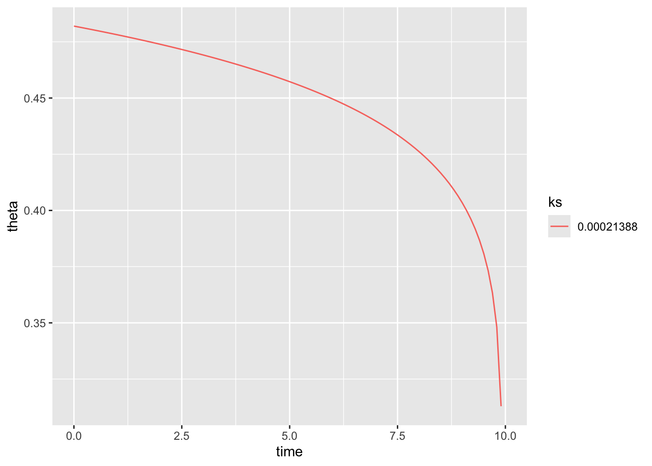
Parameters
\(K_s\): Saturated soil hydraulic conductivity \((m^3 m^{-2} yr^{-1})\) \(c\): Unitless empirical soil parameter
# Timestep
t <- seq(0,10, by = 0.01)

# Variables
theta_init <- c(theta=0)

# Model parameters
params <-
  expand_grid(theta_sat = 0.482,
            R  = 1.0,
            ks = c(40.47, 146),
            c = 4,
            b = 4) %>%
        split(., .$ks)

# Rates of change
theta_rates <- function(t, theta, params) {
  with(as.list(c(theta, params)), {

    dtheta_dt = R*(1-(theta/theta_sat)^b)-ks*(theta/theta_sat)^c

    return(list(c(dtheta_dt)))
  })
}
logistic_solution <-
map_dfr(
params,
~ode(
y = theta_init,
times = t,
func = theta_rates,
parms = .x) %>%
as.data.frame(), .id = "ks")logistic_solution %>%
ggplot(aes(time, theta, col=ks)) +
geom_line()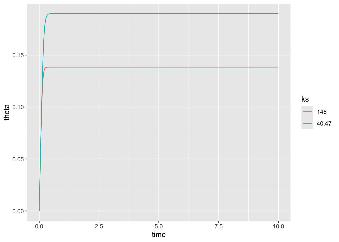
Now with climatic variability of amplitude = the annual mean rainfall
# Timestep
t <- seq(0,10, by = 0.01)

# Variables
theta_init <- c(theta=0)

# Model parameters
params <-
  expand_grid(theta_sat = 0.482,
            R  = 1.0,
            ks = c(40.47, 5550.37),
            c = 11,
            b = 4) %>%
        split(., .$ks)

# Rates of change
theta_rates <- function(t, theta, params) {
  with(as.list(c(theta, params)), {

    dtheta_dt = (R+R*sin(t/(2*pi)^-1))*(1-(theta/theta_sat)^b)-ks*(theta/theta_sat)^c

    return(list(c(dtheta_dt)))
  })
}
logistic_solution <-
map_dfr(
params,
~ode(
y = theta_init,
times = t,
func = theta_rates,
parms = .x) %>%
as.data.frame(), .id = "ks")logistic_solution %>%
ggplot(aes(time, theta, col=ks)) +
geom_line()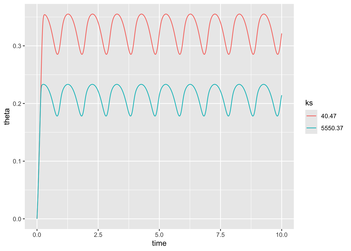
# Timestep
t <- seq(0,10, by = 0.01)

# Variables
theta_init <- c(theta=0)

# Model parameters
params <-
  expand_grid(theta_sat = 0.482,
            R  = 1.0,
            ks = c(40.47),
            c = 11,
            b = 4,
            pe = c(0.5,1,1.4),
            k = 0.46,
            LAI = 0) %>%
        split(., .$pe)


# Rates of change
theta_rates <- function(t, theta, params) {
  with(as.list(c(theta, params)), {

    dtheta_dt = R*(1-(theta/theta_sat)^b)-ks*(theta/theta_sat)^c -
    pe*(exp(-k * LAI)/(1 + exp (-12 * (theta /theta_sat - 0.5))))

    return(list(c(dtheta_dt)))
  })
}
logistic_solution <-
map_dfr(
params,
~ode(
y = theta_init,
times = t,
func = theta_rates,
parms = .x) %>%
as.data.frame(), .id = "pe")logistic_solution %>%
ggplot(aes(time, theta, col=pe)) +
geom_line()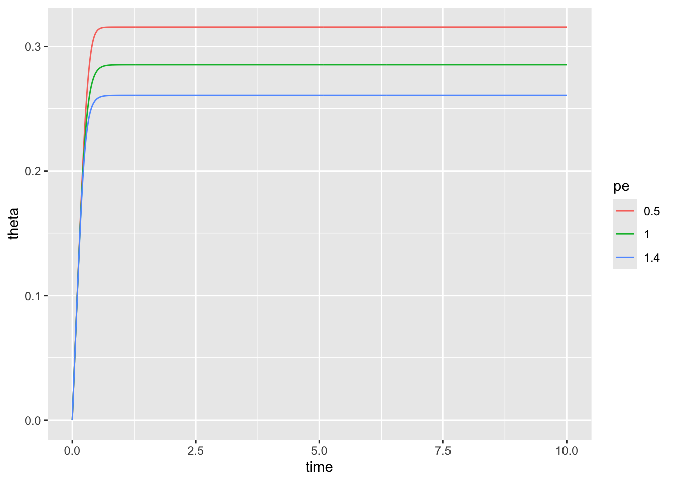
# Timestep
t <- seq(0,10, by = 0.01)

# Variables
theta_init <- c(theta=0)

# Model parameters
params <-
  expand_grid(theta_sat = 0.482,
            R  = 1.0,
            ks = c(40.47),
            c = 11,
            b = 4,
            pe = c(0.5, 1,1.4),
            k = 0.46,
            LAI = 0) %>%
        split(., .$pe)


# Rates of change
theta_rates <- function(t, theta, params) {
  with(as.list(c(theta, params)), {

    dtheta_dt = (R+R*sin(t/(2*pi)^-1))*(1-(theta/theta_sat)^b)-ks*(theta/theta_sat)^c -
    pe*(exp(-k * LAI)/(1 + exp (-12 * (theta /theta_sat - 0.5))))

    return(list(c(dtheta_dt)))
  })
}
logistic_solution <-
map_dfr(
params,
~ode(
y = theta_init,
times = t,
func = theta_rates,
parms = .x) %>%
as.data.frame(), .id = "pe")logistic_solution %>%
ggplot(aes(time, theta, col=pe)) +
geom_line()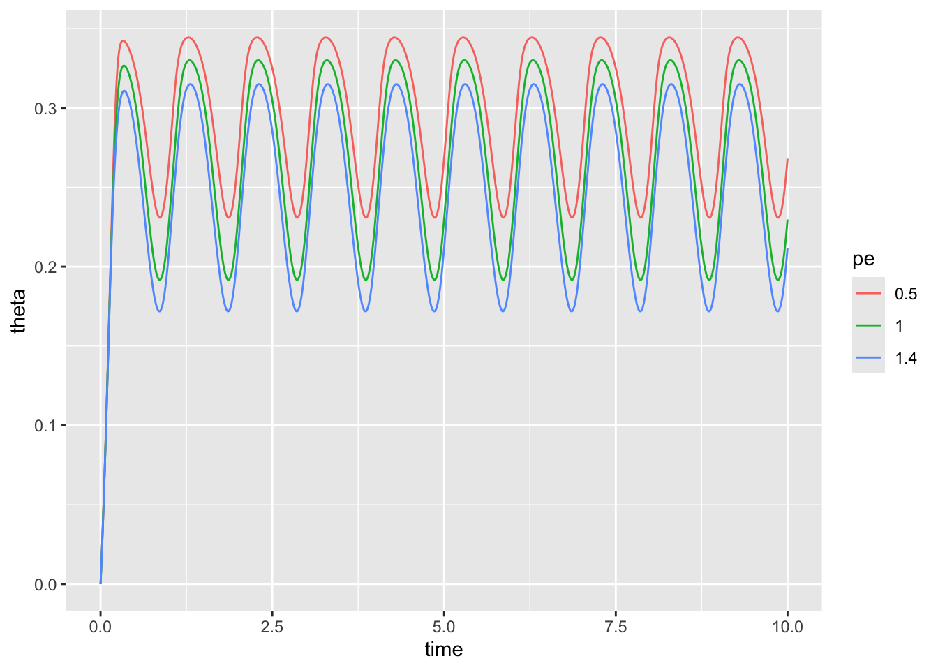
Evaporation should occur only in the top 10 cm of soil https://pure.mpg.de/rest/items/item_1781494/component/file_1786328/content
\(J\) is defined as:
\[J= -D_z(\theta_z)\frac{\delta\theta}{\delta{z}},\]
Where the diffusivity, \(D\) \((m^2 s^{-1})\) is defined as:
\[D_z(\theta_z) = \frac{K_z}{g*p_w}\frac{\delta\psi}{\delta\theta},\]
and the hydraulic conductivity \(K_d\) \((m~yr^{-1})\) is defined as:
\[K_z=K_{sat}\bigg(\frac{\theta_z}{\theta_{sat}}\bigg)^{nk}.\]
\(K_{sat}\) \((m~yr^{-1})\) and \(nk\) (unitless) are empirical parameter which vary with soil type, \(g\) is acceleration due to gravity \((9.8~m~s^{-2})\) and \(p_w\) is the density of water \((1000~kg~m^{-3})\). Finally, \(\psi\) is the soil water potential.
Because the soil water potential at a given depth is related to soil moisture content according to the following equation:
\[\psi_z=-a_\psi \theta_z^{-n_\psi},\]
where \(a_\psi\) and \(n_\psi\) are soil-dependent empirical parameters. It follows that diffusivity can be calculated in terms of soil moisture content at a given depth according to the following equation:
\[D_z(\theta_z) = \frac{K_z}{g*p_w}a_{\psi}n_{\psi}\theta_z^{-n_{\psi}-1},\]
Thus, \(J\) equals:
\[J= -\frac{K_{sat}\bigg(\frac{\theta_z}{\theta_{sat}}\bigg)^{nk}}{g*p_w}a_{\psi}n_{\psi}\theta_z^{-n_{\psi}-1}\frac{\delta\theta}{\delta{z}},\]
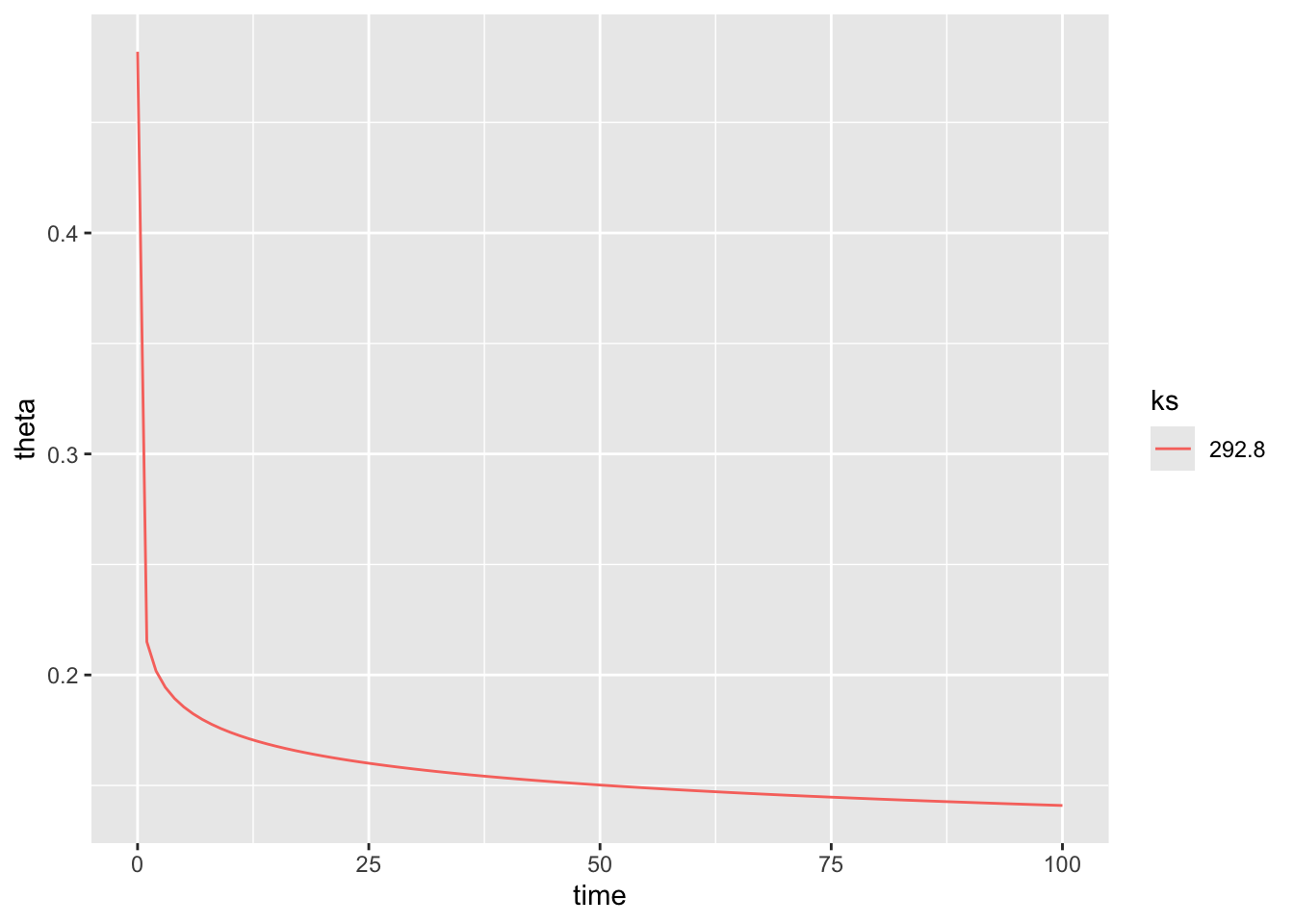
# Timestep
t <- seq(0,100, by = 1)

# Variables
theta_init <- c(theta=0.482)

# Model parameters for silty loam (Landsberg)
params <-
  expand_grid(
    #convert to day
    ksat = c(12.2*24),
    nk = 11.9,
    theta_sat = 0.482,
    g = 9.8,
    pw = 1000,
    apsi = 1.87,
    npsi = 4.5) %>%
        split(., .$ksat)

# Rates of change
theta_rates <- function(t, theta, params) {
  with(as.list(c(theta, params)), {
    soil_conductivity = ksat * (theta/theta_sat)^nk
    dpsi_dtheta = apsi * npsi * theta ^ (-npsi-1)
    # dtheta_dt = - (soil_conductivity/(g*pw))*dpsi_dtheta*((theta-0.2)/0.1)
      dtheta_dt = - (soil_conductivity)

    return(list(c(dtheta_dt)))
  })
}
logistic_solution <-
map_dfr(
params,
~ode(
y = theta_init,
times = t,
func = theta_rates,
parms = .x) %>%
as.data.frame(), .id = "ks")logistic_solution %>%
ggplot(aes(time, theta, col=ks)) +
geom_line()